PyTorch - Neural network for simple regression analysis
Regression analysis is an analysis, which allows us to find Y value for any given X values, on the basis of some (x,y) data set. For this example we will use any function with introduced extra noise.

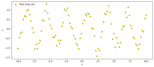
Training set is a simple SIN(x) function with introduces random noise.
Original image: 731 x 317
This picture represents our data for regression analysis with neural network. This is simple SIN(x) function with introduced noise, and we will try to build and train simple Neural Network which can predict Y for any X from this range.
Libraries for Neural Network regression analysis
We need to have torch library for modelling Neural Network and mathplotlib for visual analysis. Also initiate picture size
import torch
import matplotlib.pyplot as plt
import matplotlib
matplotlib.rcParams['figure.figsize'] = (12.0, 5.0)
Required datasets
In “real life” we will have dataset collected from some real experiments, but for training purposes we will make this dataset from simple function.
We will make ideal dataset
x_validation and y_validation - this will be ideal function, which we will use to validate our solution.
x_train and y_train - this is our train data set with introduced noise, random 10% variation to y values. Because training dataset is not ideal, we will never have perfect match between our results and validation dataset.
With unsqueeze_ method we will turn our data into proper torch format, suitable for Neural Network modelling
# target function is a simple generator of our "unknown" data
def target_function(x):
    return torch.sin(2*x)

# Generation all datasets -----------
drange = (-10, 10, 100) # data range for function (from, to, steps)
noise_level = 0.1       # noise strength 0.1 = 10%

# training set
x_train = torch.linspace(drange[0], drange[1], drange[2])
y_train = target_function(x_train)

# calculate noise for training set (to making  data more real)
noise_coef = (y_train.max()-y_train.min()) * noise_level
noise = torch.randn(y_train.shape) * noise_coef

# add noise to the data set
y_train = y_train + noise

# prepare data for NN with one data per line
x_train.unsqueeze_(1)
y_train.unsqueeze_(1)

# ideal data will be used for validation
x_validation = torch.linspace(drange[0], drange[1], drange[2])
y_validation = target_function(x_validation)
x_validation.unsqueeze_(1)
y_validation.unsqueeze_(1)
# ------Dataset preparation end--------:
Defining Neural Network class
Now we need to describe our Neural Network model. We build is as a class with parent from torch.nn.Module. This class contains initialisation with description of all layers of our Neural Network and one step forward technique, which describes the way of using these layers.
It is necessary to mention following points: initialisation function will create Neural Network for some number of neurons in the layer.
It is also necessary to describe every network layer. In this example we make 3 layers.
1 fully connected (linear layer), fc1, which takes one entering value with one neurone and spread it to required number on neurones.
2 second layer act1 - activation function. You can choose between most popular Sigma activation, Pseudo Linear activation or ArcTan activation functions. For example, check hoe hyperbolic tangent activation function for regression with different numbers of neurons:
3 third layer – again linear layer to combine all activation results into one neurone for output.
It is important to mention, that it is possible to combine as many layers as you need, but this configuration will only be defined once for this network
Secondly, it is necessary to identify, how this layers are linked with each other during one step of network calculation. I’ve show two ways of doinf it with simple and more complicated “pythonish” style of writing.
class RegressionNet(torch.nn.Module):
    # initialisation of NN
    def __init__(self, n_hidden_neurons):
        # initialize parent
        super(RegressionNet, self).__init__()

        # describe NN layers
        # first layer: 1 entrance neuron; n - exit neurines
        # Fully connected layer (linear)
        self.fc1  = torch.nn.Linear(1, n_hidden_neurons)
        # second layer: sigma activation function
        self.act1 = torch.nn.Sigmoid()

        # few examples of other activation functions
        # second layer: semi linear activation function
        # self.act1 = torch.nn.ReLU()
        # second layer: ArcTan activation function
        # self.act1 = torch.nn.Tanh()

        # third layer: exit - one neurone
        self.fc2 = torch.nn.Linear(n_hidden_neurons, 1)

    def forward(self, x): # way of applying layers of neurons
        # use all layers
        for f in ['fc1', 'act1', 'fc2']:
            x = getattr(self, f)(x)
        '''
        # this is equivalent to
            x = self.fc1(x)
            x = self.act1(x)
            x = self.fc2(x)
        '''
        return x
Loss function
Loss function – function which will calculate our metric to see how far we are from our target. It is necessary to understand, that we are optimizing Neural Network wights (parameters) to minimize loss function. It is possible to use any metric for our loss function. For example mean square ot absolute (Manhattan) metrics are good enough for our case.
def loss(pred, target):
    # metric to check the difference between target and prediction
    # absolute = abs(pred - target)
    square = (pred - target)**2
    return square.mean()
Manual defining of starting parameters
Every Neural Network, after defining its structure, requires to have some initial parameters to start.
For our model it is important to identify total number of neurones.
Too small number of neurones can give very poor prediction. Too much neurones can give over-prediction.
Number of epoch, or number of neural network optimisation weights optimisation cycles. Generally we should achieve best matching with our validation set, but it is necessary to have a balance and understand that this kind of optimisation can be very long.
Initial step of gradient or Learning Rate – this is depends on our task and Neural Network structures, but in fast, if we will use very big amount, our solution will be spiky – with a lot of disturbances and sometimes with chance never to achieve good results. If we will choose very small initial step, then it can take very long time (too many cycles) to find final result.
total_neurons = 50 # total number of neurones in the hidden layer
total_epoch   = 5000 # total number of training epoch
lr_start      = 0.01 # first step of gradient (learning rate)
Initializing Neural Network
Now we need to initialize of Neutral Network with given number of neurones. And we need to specify, which optimizer we will use. There are a lot of different optimizers, utilizing different techniques for gradient minimization. I do advise to use Adam as a first try (can try simple gradient minimization SGD). And don't forget to tell, what is your initial step for this optimisation.
Also we will create data structure for storing metric of our progress.
# create network wit given number of neurons
NN = RegressionNet(total_neurons)

# define optimizer for NN
# We use "ADAM" gradient optimization algorithm
# Also, we optimizing NN parameters! (not x or y!)
optimizer = torch.optim.Adam(NN.parameters(), lr=lr_start)

# data for monitoring loss improvement
loss_history = [[0,0] for i in range(total_epoch)]
Doing optimization itself
It is important to remember to reset optimizer parameters before each new epoch (cycle) with function zero_grad(). Otherwise you will use optimizer parameters from previous step
Next step, from our data set we calculate prediction forward. Then we calculate our loss function to find how far we are, and update our loss_history log
Then we recalculate this step backwards and optimizer make step. This is our full cycle of calculation.
for e in range(total_epoch):
    print(e, end='\r') # output for progress monitoring
    optimizer.zero_grad() # reset optimizer (don;t forget to do it!)

    y_pred = NN.forward(x_train)          # calculate prediction
    loss_val = loss(y_pred, y_train)       # calculate loss function (scalar)

    loss_history[e] = [e, loss_val.data.numpy().tolist()]

    loss_val.backward()                    # do step back

    optimizer.step()                       # ask optimizer to do one step
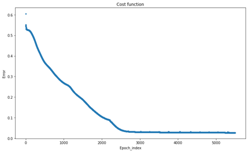
Changes of Cost Function during our optimisation process
Original image: 721 x 442
You can see how loss function is reducing over each epoch cycle
To plot this loss function over epochs you can use matplotlib and our structure loss_history which we create during our optimisation.
When presenting data structure from tensor it is necessary to convert it to numpy structure.
# plot loss function history
plt.plot([row[0] for row in loss_history], [row[1] for row in loss_history], '.')
plt.title(label='Loss function')
plt.xlabel('Epoch_index')
plt.ylabel('Error');
plt.show()
Final prediction
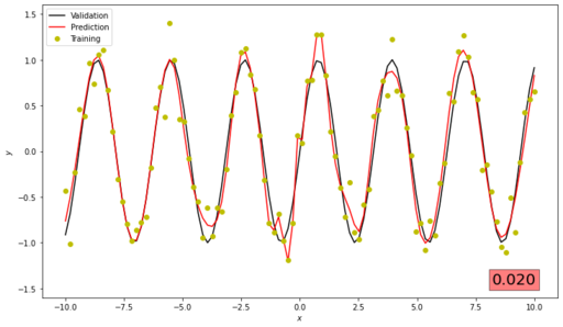
Now we can use our trained Neural Network to predict values and compare them with our validation datasets loss(NN.forward(x_validation), y_validation).item() and draw the final graphs
# function for presentation
def predict(net, x, y):
    y_pred = net.forward(x)

    plt.plot(x.numpy(), y.numpy(), 'o', label='Groud truth')
    plt.plot(x.numpy(), y_pred.data.numpy(), 'o', c='r', label='Prediction');
    plt.plot(x.numpy(), y_train.data.numpy(),'o', c='y', label='Train');
    plt.legend(loc='upper left')
    plt.xlabel('$x$')
    plt.ylabel('$y$')
    plt.show()
predict(NN, x_validation, y_validation)
Our graph should looks like this one. If the correspondence is not good enough, then we need to use different parameters to train our network

Changes of Loss Function during our optimisation process
Original image: 731 x 425
Full code for regression with neural network
Complete code in one place. Run this code and if it is working – you can modify it to adjust to your task.
import torch
import matplotlib.pyplot as plt
plt.rcParams["figure.figsize"] = (12,7)

# target function is a simple generator of our "unknown" data
def target_function(x):
    return torch.sin(2*x)
# Generation all datasets -----------
drange = (-10, 10, 100) # data range for function (from, to, steps)
noise_level = 0.1 # noise strength 0.1 = 10%
# training set
x_train = torch.linspace(drange[0], drange[1], drange[2])
y_train = target_function(x_train)
# calculate noise for training set (to making data more real)
noise_coef = (y_train.max()-y_train.min()) * noise_level
noise = torch.randn(y_train.shape) * noise_coef
# add noise to the data set
y_train = y_train + noise
# prepare data for NN with one data per line
x_train.unsqueeze_(1)
y_train.unsqueeze_(1)
# ideal data will be used for validation
x_validation = torch.linspace(drange[0], drange[1], drange[2])

y_validation = target_function(x_validation)
x_validation.unsqueeze_(1)
y_validation.unsqueeze_(1)
# ------Dataset preparation end--------:

class RegressionNet(torch.nn.Module):
    # initialisation of NN
    # initialize neural network with n hidden neurons
    def __init__(self, n_hidden_neurons):
        # initialize parent
        super(RegressionNet, self).__init__()

        # describe NN layers
        # first layer: 1 entrance neuron; n - exit neurines
        # Fully connected layer (linear)
        self.fc1  = torch.nn.Linear(1, n_hidden_neurons)

        # second layer: sigma activation function
        self.act1 = torch.nn.Sigmoid()

        # third layer: exit - one neurone
        self.fc2 = torch.nn.Linear(n_hidden_neurons, 1)

    def forward(self, x): # way of applying layers of neurons
        # use all layers
        for f in ['fc1', 'act1', 'fc2']:
            x = getattr(self, f)(x)
        return x

def loss(pred, target):
    # metric to check the difference between target and prediction
    # absolute = abs(pred - target)
    square = (pred - target)**2
    return square.mean()


total_neurons = 50 # total number of neurones in the hidden layer
total_epoch   = 5500 # total number of training epoch
lr_start      = 0.01 # first step of gradient (learning rate)


NN = RegressionNet(total_neurons)

# define optimizer for NN
# We use "ADAM" gradient optimization algorithm
# Also, we optimizing NN parameters! (not x or y!)
optimizer = torch.optim.Adam(NN.parameters(), lr=lr_start)

# data for monitoring loss improvement
loss_history = [[0,0] for i in range(total_epoch)]


for e in range(total_epoch):
    print(e, end='\r') # output for progress monitoring
    optimizer.zero_grad() # reset optimizer (don;t forget to do it!)

    y_pred = NN.forward(x_train)          # calculate prediction
    loss_val = loss(y_pred, y_train)       # calculate loss function (scalar)

    loss_history[e] = [e, loss_val.data.numpy().tolist()]

    loss_val.backward()                    # do step back

    optimizer.step()                       # ask optimizer to do one step


# plot loss function history
plt.plot([row[0] for row in loss_history], [row[1] for row in loss_history], '.')
plt.title(label='Cost function')
plt.xlabel('Epoch_index')
plt.ylabel('Error');
plt.show()

# graphical output
def predict(net, x, y):
    y_pred = net.forward(x)

    rms = loss(net.forward(x_validation), y_validation).item()

    plt.ylim(-1.6, 1.6)
    plt.plot(x.numpy(), y.numpy(), c='k', label='Validation', ls='-')
    plt.plot(x.numpy(), y_pred.data.numpy(), c='r', label='Prediction', ls='-');
    plt.plot(x.numpy(), y_train.data.numpy(),'o', c='y', label='Training');
    plt.legend(loc='upper left')
    plt.xlabel('$x$')
    plt.ylabel('$y$')
    plt.text(8.2, -1.45, f'{rms:.3f}', fontsize = 20,
         bbox = dict(facecolor = 'red', alpha = 0.5))
    plt.show()

predict(NN, x_validation, y_validation)
Published: 2022-06-02 03:28:55
Updated: 2022-06-18 02:45:14