Plotting of Interactive Electric field due to point charges with Matplotlib
This tutorial will be more focused on Python coding, rather than on the physics of the process, because all physics was described in the previous part of calculating of electric field potential and intensity due to point charges, or in the video about it
Here I will give mainly information, about how to use Matplotlib Widgets.
Initial description of domain, functions and plot
Domain description
As usual, the first step in any proper MHD and EMHD calculations is to generate domain for calculations. After loading all required libraries, of course.
For convenience, all field variables will be stored in one dictionary D - it will make it easier to send to some functions
import numpy as np
import matplotlib.pyplot as plt
from matplotlib.widgets import Slider, CheckButtons, RadioButtons

xrange = [-1., 1.]   # left and right coordinates of square domain (x==y)
step = 40            # Number of cells in the domain in any axis
qrange = [-10., 10.] # max and min values for charge
NQ = 4               # Number of charges

D = {}  # domain description
D['X'], D['Y'] = np.meshgrid(xlist, ylist)
D['Ex'] = np.zeros_like(D['X'])
D['Ey'] = np.zeros_like(D['X'])
D['V'] = np.zeros_like(D['X'])
D['E'] = np.zeros_like(D['X'])
D['Q'] = np.random.uniform(low=qmin, high=qmax, size=(NQ, 3))
How to generate randomply places charges (last line in the code) described here: how to make random array
Electric field calculations
Second, very important step is to make function for electric field calculations. To make calculations slightly faster, I’ve use non-standard distance calculating. I’ve apply power of (3/2) and it save me one power calculation for a full domain. Profit!!! But it will make code more confusing and should only used when it is really necessary
def addPointCharge2D(V, Ex, Ey, X, Y, q):
    # Add one charge to the field
    r2 = ((X - q[0]) ** 2 + (Y - q[1]) ** 2) ** (3 / 2)
    Ex += q[2] * (X - q[0]) / r2  # Electric field (x)
    Ey += q[2] * (Y - q[1]) / r2  # Electric field (y)
    V += q[2] / r2 ** (1 / 3.)
    return V, Ex, Ey

def ElectricField(E, Ex, Ey, V, X, Y, Q):
    # Calculate for all charges
    Ex *= 0
    Ey *= 0
    V *= 0
    for q in Q:
        addPointCharge2D(V, Ex, Ey, X, Y, q)
    E[:] = np.log((Ex ** 2 + Ey ** 2)) * 0.5
    return E, Ex, Ey, V

ElectricField(**D) # Calculate E field for initial charge combination
Plotting out results
After calculation Electric field intensity and potential energy, it is convenient to make it plot. But before plotting we will create control variables, to control which information we will plot. This is very important, because later, when we will use widgets to modify something, these control variable will be used.
P = {}  # plot description
P['plt_type'] = ['Position', 'Field', 'Lines']  # type of shown information
P['plt_active'] = [True, True, True]            # Show or not switches
P['ColorBar'] = None                            # initial colorbar
P['field_type'] = ['V', 'E']                    # available field for plotting
P['VE'] = False                                 # show vector field
P['levelE'] = np.linspace(-1, 10, 100)          # range for Efield colorbar
P['levelV'] = np.linspace(-150, 150, 100)       # range for Vfield colorbar
P['Qactive'] = 0                                # Current active charge
P['line_density_range'] = [0.1, 2.0]            # Range of possible line densities
P['line_density'] = 0.4                         # current line density
P['fig'], P['ax'] = plt.subplots(figsize=(6, 5))
And at the last line we are creating subplot itself and matplotlib.axes.Axes object for all plotting. Also we physically define the size of the picture in inches (6, 5).
After defining all controls, we can make a function to plot all graphical information according to these controls:
def el_plot(P, D):
    P['ax'].clear()

    if P['plt_active'][0]:
        # Position
        P['ax'].scatter(D['Q'][:, 0], D['Q'][:, 1], c=np.where(D['Q'][:, 2] < 0, 'b', 'r'))
        for i, txt in enumerate(D['Q']):
            P['ax'].annotate(f'({i + 1}):{txt[2]:.1f}', xy=(D['Q'][i, 0], D['Q'][i, 1]),
                             xytext=(D['Q'][i, 0] + 0.02, D['Q'][i, 1] + 0.02),
                             color='black', fontsize='12')
    if P['plt_active'][1]:
        # Field
        if P['VE']:
            P['ax'].set_title("Electric Field Intensity, E")
            cp = P['ax'].contourf(D['X'], D['Y'], D['E'], levels=P['levelE'], cmap='jet')
        else:
            P['ax'].set_title("Electric Potential energy, V")
            cp = P['ax'].contourf(D['X'], D['Y'], D['V'], levels=P['levelV'], cmap='seismic')
        if P['ColorBar']:
            P['ColorBar'].remove()
        P['ColorBar'] = P['fig'].colorbar(cp, ax=P['ax'])

    if P['plt_active'][2]:
        # Lines
        P['ax'].streamplot(D['X'], D['Y'], D['Ex'], D['Ey'], color='black', linewidth=0.5,
                           density=P['line_density'], arrowstyle='->', arrowsize=1.0)

    plt.draw()
    return None
It is important to mention, that before every plotting we clear all previously plotted information P['ax'].clear() and also we remove ColourBar before plotting new one. Also for the very first colourbar plotting we have nothing to remove.
After defining function for plotting, we can call it, but before it we need to adjust position of the sublot to make some space for future widgets and also forcedly restrict plotting area – this is necessary to avoid automatic rescaling in the future.
plt.subplots_adjust(left=0.20, bottom=0.35)
plt.xlim(xrange[0], xrange[1])
plt.ylim(xrange[0], xrange[1])

el_plot(P, D)
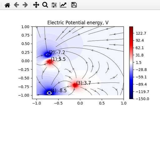
electric Potential Energy V, calculated for 4 randomly placed charges. Some space is allocated for Widgets.
Original image: 588 x 524
Plot control with Matplotlib Widgets
When the plot with initial data is ready and it working perfectly, it is a good time to add widgets to interactively change some parameters.
Sliders
Sliders are very convenient, when it is necessary to smoothly change some of the parameters. For example, in our case, sliders will be ideal for modifying position of charges and charge value. Also it is very convenient to modify some of the plot parameters, like line density.
To make slider, it is necessary to allocate physical space with Axis for it. This physical space should be allocated in inches
ax_x = plt.axes([0.20, 0.25, 0.55, 0.05]) # Left, bottom, width, height (Horizontal)
ax_y = plt.axes([0.07, 0.35, 0.05, 0.53]) # Left, bottom, width, height (VERTICAL SLIDER)
ax_q = plt.axes([0.20, 0.20, 0.55, 0.05]) # Left, bottom, width, height (Horizontal)
ax_d = plt.axes([0.20, 0.15, 0.55, 0.05]) # Left, bottom, width, height (Horizontal)
In this example, four spaces are allocated, and it is easy to see, that ax_y is vertical. At he next step it is necessary to run constructor to initialize sliders for these areas
s_x = Slider(ax_x, 'x', qmin[0], qmax[0], valinit=D['Q'][P['Qactive']][0])
s_y = Slider(ax_y, 'y', qmin[1], qmax[1], valinit=D['Q'][P['Qactive']][1],
             orientation="vertical")
s_q = Slider(ax_q, 'q', qmin[2], qmax[2], valinit=D['Q'][P['Qactive']][2])
s_d = Slider(ax_d, 'l', P['line_density_range'][0], P['line_density_range'][1],
             valinit=P['line_density'])
For Slider constrictor it is necessary to provide location, name, range of values and initial value, where slider wheel will be located. Initial position will be remembered with an option to reset it and also market with thin red line. It is possible to remove this red line.
It is depend on the task you solving, how important to keep these red lines. I prefer to remove them
s_x.vline._linewidth = 0
s_y.hline._linewidth = 0 # Be careful – this line is horizontal!
s_q.vline._linewidth = 0
s_d.vline._linewidth = 0
At the next step it is necessary to define function, which will respond to the changes of the sliders
def slider_update(val, P, D):
    # variable q is for making writing shorter
    q = D['Q'][P['Qactive']]
    # reading positions of all sliders
    q[0] = s_x.val # position of s_x slider
    q[1] = s_y.val # position of s_y slider
    q[2] = s_q.val
    P['line_density'] = s_d.val
    # recalculation of the plot in accordance with the new positions
    # recalculation
    ElectricField(**D)
    # redraw plot with the new data
    # output
    el_plot(P, D)
This function will be called upon any changes in the slider position and value will be passed to this function by default. To pass more parameters it is necessary to use lambda call.
The standard way of using this function – read values from sliders (val), then recalculated displayed values and then redraw the plot.
To call this function, it is necessary to use on_changed method to appropriate slider. In this code fragment, I will call use this method with lambda activation of the update function
s_x.on_changed(lambda new_val: slider_update(new_val, P, D))
s_y.on_changed(lambda new_val: slider_update(new_val, P, D))
s_q.on_changed(lambda new_val: slider_update(new_val, P, D))
s_d.on_changed(lambda new_val: slider_update(new_val, P, D))
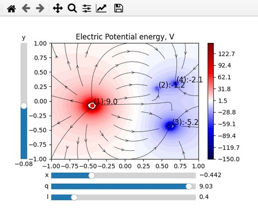
The result of this code you can see here:

Electric Potential Energy V, calculated for 4 randomly placed charges with sliders, which allow to change location and charge of the first charge on this plot.
Original image: 589 x 509
Checkbutton
Checkbutton block allow to set in ON and OFF position some variables. It is very convenient to keep they values as a boolean variable, to make switching very simple. Just a reminder – to change boolean value to an apposite, use command not.
# Define location of the check box
ax_qfl = plt.axes([0.03, 0.17, 0.13, 0.13])
# Initiate check box
chxbox = CheckButtons(ax_qfl, P['plt_type'], P['plt_active'])
Fot checkbox initiation it is necessary to provide location of this checkbox, list of options and list of boolean states of these switches.
def qfl_select(label, P, D):
    # change clicked checkbutton
    index = P['plt_type'].index(label)
    P['plt_active'][index] = not P['plt_active'][index]

    # output
    el_plot(P, D)
Function acted upon call of checkbox status change is a bit inconvenient. As a value of checkbox change is receive the name of the box changed. Therefore all names should be unique and also to work out number of the box clicked, you need to use function index
Call of this function upon any changes is pretty standard for any Matplotlib Widgets:
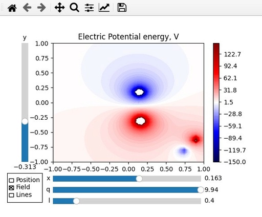
chxbox.on_clicked(lambda new_select: qfl_select(new_select, P, D))In this case again, lambda call was used to pass more arguments. The result will be similar to this one:

Electric Potential Energy V, calculated for 4 randomly placed charges with sliders and checkbox. Checkbox allow to do not display charge names and electric field lines.
Original image: 584 x 484
Radiobuttons
Radiobutton allow to have a box of switches with only one switch on positive and all other in the negative state. The coding of radiobutton is pretty similar to those for checkbox. As a default value, when changed, the function receive the name of activated button. If you have only two buttons, it is possible to do not use any labes and just change the status of this radiobutton to opposite.
ax_ev = plt.axes([0.85, 0.20, 0.10, 0.10])  # left, bottom, width, height values
rbutton1 = RadioButtons(ax_ev, P['field_type'])

def ev_select(label, P, D):
    # swap clicked rbutton
    P['VE'] = not P['VE']

    # output
    el_plot(P, D)

rbutton1.on_clicked(lambda new_select: ev_select(new_select, P, D))
In this case only two options are available and label - label of switched button is not used.
In the next part of the code, radiobutton will have few buttons equal to number of charges in the system. Therefore the size of the space will be proportional to number of charges
ax_qs = plt.axes([0.01, 0.40, 0.06, 0.03 * NQ])  # left, bottom, width, height values
rbutton2 = RadioButtons(ax_qs, range(1, NQ + 1), active=P['Qactive'])
It is also necessary to report active button, otherwise by default it will use first button in the list.
Question: Is it possible to place all buttons with horizontal alinement's?
Answer: No. Standard tools do not provide this option at the moment. If it is necessary to do this, you need to allocate every button separately within the same axes.
In the next response function I will change active change, and reset sliders position to the new value
def q_select(label, P, D):
    P['Qactive'] = int(label) - 1
    q = D['Q'][P['Qactive']]

    s_x.eventson = False
    s_y.eventson = False
    s_q.eventson = False
    s_x.set_val(q[0])
    s_y.set_val(q[1])
    s_q.set_val(q[2])
    s_x.eventson = True
    s_y.eventson = True
    s_q.eventson = True

rbutton2.on_clicked(lambda new_select: q_select(new_select, P, D))
In this q_select function reading of the clicked option is standard. But because labels are integer and equal to the charge number +1 it is very easy to work our real charge numbers.
The position of slider can easily be changed with method set_val applied to the correspondent slider. But when the position of slider changed, it is important to deactivate it, otherwise it will cause changes in the system by calling slider on_change function.
To deactivate slider for some time, use changing of the eventson variable from True to False and back at the end of changing. But be careful eventson is not documented feature at he moment and can be changed without further notice.
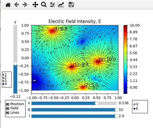
The result of all these changes will be similar to this one:

Electric Intensity Field E, calculated for 4 randomly placed charges with Sliders, Radiobuttons and Checkbuttons. These widgets allow to change the location and charge of all charges and change all information displayed.
Original image: 593 x 495
Fill final code for Plotting of Interactive Electric field due to point charges with Widgets
import numpy as np
import matplotlib.pyplot as plt
from matplotlib.widgets import Slider, CheckButtons, RadioButtons

def addPointCharge2D(V, Ex, Ey, X, Y, q):
    r2 = ((X - q[0]) ** 2 + (Y - q[1]) ** 2) ** (3 / 2)
    Ex += q[2] * (X - q[0]) / r2  # Electric field (x)
    Ey += q[2] * (Y - q[1]) / r2  # Electric field (y)
    V += q[2] / r2 ** (1 / 3.)
    return V, Ex, Ey


def ElectricField(E, Ex, Ey, V, X, Y, Q):
    Ex *= 0
    Ey *= 0
    V *= 0
    for q in Q:
        addPointCharge2D(V, Ex, Ey, X, Y, q)
    E[:] = np.log((Ex ** 2 + Ey ** 2)) * 0.5
    return E, Ex, Ey, V


xrange = [-1., 1.]   # left and right coordinates of square domain (x==y)
step = 40            # Number of cells in the domain in any axis
qrange = [-10., 10.] # max and min values for charge
NQ = 4               # Number of charges

P = {}  # plot description
P['plt_type'] = ['Position', 'Field', 'Lines']  # type of shown information
P['plt_active'] = [True, True, True]            # Show or not switches
P['ColorBar'] = None                            # initial colorbar
P['field_type'] = ['V', 'E']                    # available field for plotting
P['VE'] = False                                 # show vector field
P['levelE'] = np.linspace(-1, 10, 100)          # range for Efield colorbar
P['levelV'] = np.linspace(-150, 150, 100)       # range for Vfield colorbar
P['Qactive'] = 0                                # Current active charge
P['line_density_range'] = [0.1, 2.0]            # Range of possible line densities
P['line_density'] = 0.4                         # current line density

xlist = np.linspace(xrange[0], xrange[1], step)
ylist = np.linspace(xrange[0], xrange[1], step)
qmin = [xrange[0], xrange[0], qrange[0]]
qmax = [xrange[1], xrange[1], qrange[1]]

D = {}  # domain description
D['X'], D['Y'] = np.meshgrid(xlist, ylist)
D['Ex'] = np.zeros_like(D['X'])
D['Ey'] = np.zeros_like(D['X'])
D['V'] = np.zeros_like(D['X'])
D['E'] = np.zeros_like(D['X'])
D['Q'] = np.random.uniform(low=qmin, high=qmax, size=(NQ, 3))

ElectricField(**D)


############ INITIAL PLOT

def el_plot(P, D):
    P['ax'].clear()

    if P['plt_active'][0]:
        # Position
        P['ax'].scatter(D['Q'][:, 0], D['Q'][:, 1], c=np.where(D['Q'][:, 2] < 0, 'b', 'r'))
        for i, txt in enumerate(D['Q']):
            P['ax'].annotate(f'({i + 1}):{txt[2]:.1f}', xy=(D['Q'][i, 0], D['Q'][i, 1]),
                             xytext=(D['Q'][i, 0] + 0.02, D['Q'][i, 1] + 0.02),
                             color='black', fontsize='12')
    if P['plt_active'][1]:
        # Field
        if P['VE']:
            P['ax'].set_title("Electric Field Intensity, E")
            cp = P['ax'].contourf(D['X'], D['Y'], D['E'], levels=P['levelE'], cmap='jet')
        else:
            P['ax'].set_title("Electric Potential energy, V")
            cp = P['ax'].contourf(D['X'], D['Y'], D['V'], levels=P['levelV'], cmap='seismic')
        if P['ColorBar']:
            P['ColorBar'].remove()
        P['ColorBar'] = P['fig'].colorbar(cp, ax=P['ax'])

    if P['plt_active'][2]:
        # Lines
        P['ax'].streamplot(D['X'], D['Y'], D['Ex'], D['Ey'], color='black', linewidth=0.5,
                           density=P['line_density'], arrowstyle='->', arrowsize=1.0)

    plt.draw()
    return None


P['fig'], P['ax'] = plt.subplots(figsize=(6, 5))

plt.subplots_adjust(left=0.20, bottom=0.35)
plt.xlim(xrange[0], xrange[1])
plt.ylim(xrange[0], xrange[1])

el_plot(P, D)

####################### CONTROL
####################### SLIDERS- X, Y, Q, line density

ax_x = plt.axes([0.20, 0.25, 0.55, 0.05])
ax_y = plt.axes([0.07, 0.35, 0.05, 0.53])
ax_q = plt.axes([0.20, 0.20, 0.55, 0.05])
ax_d = plt.axes([0.20, 0.15, 0.55, 0.05])

s_x = Slider(ax_x, 'x', qmin[0], qmax[0], valinit=D['Q'][P['Qactive']][0])
s_x.vline._linewidth = 0

s_y = Slider(ax_y, 'y', qmin[1], qmax[1], valinit=D['Q'][P['Qactive']][1],
             orientation="vertical")
s_y.hline._linewidth = 0

s_q = Slider(ax_q, 'q', qmin[2], qmax[2], valinit=D['Q'][P['Qactive']][2])
s_q.vline._linewidth = 0

s_d = Slider(ax_d, 'l', P['line_density_range'][0], P['line_density_range'][1],
             valinit=P['line_density'])
s_d.vline._linewidth = 0


def slider_update(val, P, D):
    q = D['Q'][P['Qactive']]

    q[0] = s_x.val
    q[1] = s_y.val
    q[2] = s_q.val
    P['line_density'] = s_d.val

    # recalculation
    ElectricField(**D)

    # output
    el_plot(P, D)


s_x.on_changed(lambda new_val: slider_update(new_val, P, D))
s_y.on_changed(lambda new_val: slider_update(new_val, P, D))
s_q.on_changed(lambda new_val: slider_update(new_val, P, D))
s_d.on_changed(lambda new_val: slider_update(new_val, P, D))

####################### CheckButton - Q, Field, Lines selector

ax_qfl = plt.axes([0.03, 0.17, 0.13, 0.13])

chxbox = CheckButtons(ax_qfl, P['plt_type'], P['plt_active'])


def qfl_select(label, P, D):
    # change clicked checkbutton
    index = P['plt_type'].index(label)
    P['plt_active'][index] = not P['plt_active'][index]

    # output
    el_plot(P, D)


chxbox.on_clicked(lambda new_select: qfl_select(new_select, P, D))

####################### RadioButton - E/V selector

ax_ev = plt.axes([0.85, 0.20, 0.10, 0.10])  # left, bottom, width, height values
rbutton1 = RadioButtons(ax_ev, P['field_type'])


def ev_select(label, P, D):
    # swap clicked rbutton
    P['VE'] = not P['VE']

    # output
    el_plot(P, D)


rbutton1.on_clicked(lambda new_select: ev_select(new_select, P, D))

####################### RadioButton - Q selector

ax_qs = plt.axes([0.01, 0.40, 0.06, 0.03 * NQ])  # left, bottom, width, height values
rbutton2 = RadioButtons(ax_qs, range(1, NQ + 1), active=P['Qactive'])


def q_select(label, P, D):
    P['Qactive'] = int(label) - 1
    q = D['Q'][P['Qactive']]

    s_x.eventson = False
    s_y.eventson = False
    s_q.eventson = False
    s_x.set_val(q[0])
    s_y.set_val(q[1])
    s_q.set_val(q[2])
    s_x.eventson = True
    s_y.eventson = True
    s_q.eventson = True

rbutton2.on_clicked(lambda new_select: q_select(new_select, P, D))

plt.show()
Published: 2022-09-25 19:48:52
Updated: 2022-09-25 19:51:07