Linear regression for approximate solution of linear equation
This is practical task from many real experiments. If we have two, linearly related values and we need to find this relation. But from the experiment we only knows the few pairs of values, and furthermore, these pairs are not measured precisely, but with some errors. We need to find the original linear relation between these two values.
Lets for example consider these data from equation y = k*x + b:
| x | 0 | 1 | 2 | 3 |
| y | 0 | 1 | 0 | 3 |
As you can see, these data are not ideal and can’t be approximated by one line, but we need to do it. The easiest way is to calculate minimal square distance between them
Manual solution of approximate linear equation

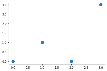
This is our original data, which we need to use for finding best line going through them
So, we need to find W1 and W0 from equation y'=W1*x + W0 with minimal square distance between y' from our calculations and y from experiment.
Speaking mathematically, we need to find the minima of the function
L(W1, W0) = Σ(W1*xi + W0 - yi)2
To find the minima, we need to solve two equations in partial derivatives
∂L/∂W1 = 0; ∂L/∂W0 = 0
or
∂/∂W1Σ(W1*xi + W0 - yi)2 = 0; ∂/∂W0Σ(W1*xi + W0 - yi)2 = 0;
For understanding of all equations, let’s do it manually here with immediate substitution of our table data:
L = (W0)2 + (W1 + W0 - 1)2 + (2*W1 + W0)2 + (3*W1 + W0 - 3)2 = 14*W21 + 4*W20 + 10 + 12*W1*W0 - 20*W0 - 8*W0;
Now we can take partial derivatives:
∂L/∂W1 = 28*W1 + 12*W0 - 20 = 0
∂L/∂W0 = 12*W1 + 8*W0 - 8 = 0
and we need to solve this system of equations.
W1 = 0.8; W0 = -0.2
How to solve the system of linear equations you can read here.

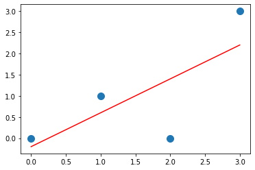
Our best fitted line is y = 0.8*x – 0.2.
Now, when we understand all mathematical operation, staying behind this procedure, we can use some python tools to solve this task
Numpay method of solving approximate systems numpy.linalg.lstsq
import numpy as np
x = np.array([0, 1, 2, 3])
y = np.array([0, 1, 0, 3])
We need to rewrite our line equation y=W1*x + W0 as y = Ap, where A = [[x 1]] and p = [[W1], [W0]], and then solve it:
A = np.vstack([x, np.ones(len(x))]).T
print(A) # to see what it is inside
#[[0. 1.]
# [1. 1.]
# [2. 1.]
# [3. 1.]]
(w1,w0) = np.linalg.lstsq(A, y, rcond=None)[0]
print(w1,w0) # 0.7999999999999997 -0.19999999999999904
which is very close to our manual solution.
Sclearn method of solving approximate systems
Basically, sclearn do the same procedure. The only difference, you need to prepare data in slightly different format. It is better to prepare data in numpy array again for easy manipulation. For linear_model.fit procedure you need to prepare data in the following format: x = [[0],[1],[2],[3]], y = [0,1,0,3]
Easiest way id to reshape X with parameters (-1, 1)
import numpy as np
from sklearn import linear_model as lm
lr = lm.LinearRegression()
x = np.array([0, 1, 2, 3])
y = np.array([0, 1, 0, 3])
x=x.reshape(-1, 1)
lr.fit(x, y)
w1 = lr.coef_[0]
w0 = lr.intercept_
print(w1,w0) # 0.7999999999999998 -0.19999999999999973
Performance comparison between Sclearn and numpy

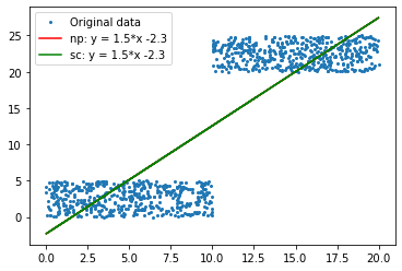
Calculation of the best fitted line with numpy.linalg.lstsq (green) and linear_model.fit (red). Both methods give the same results y = 1.5x – 2.3. They are so close that you can’t see the red line.
To calculate the time difference between these two functions I’ve create two x,y dataset with 5000 points (only 500 are shown on the picture) and solve it 10000 times with numpy and sclearn
import numpy as np
from sklearn import linear_model as lm
import datetime
# create random arrays with definetely present solution
x1 = np.random.rand(5000)*10
x2 = np.random.rand(5000)*10+10
x = np.concatenate([x1,x2])

y1 = np.random.rand(5000)*5
y2 = np.random.rand(5000)*5+20
y = np.concatenate([y1,y2])

# numpy solution
def nps(x,y):
    A = np.vstack([x, np.ones(len(x))]).T
    (w1,w0) = np.linalg.lstsq(A, y, rcond=None)[0]
    return(w1,w0)

# sklearn solution
def sks(x,y):
    xr=x.reshape(-1, 1)
    lr.fit(xr, y)
    (w1, w0) = (lr.coef_[0], lr.intercept_)
    return(w1,w0)

start_time = datetime.datetime.now()
for i in range(10000):
    (nw1, nw0) = nps(x,y)
end_time = datetime.datetime.now()
print("numpy time = ", end_time - start_time)

start_time = datetime.datetime.now()
for i in range(10000):
    (sw1, sw0) = sks(x,y)
end_time = datetime.datetime.now()
print("sklearn time = ", end_time - start_time)
The result is pretty predictable, numpy is almost 3 times faster than sklearn.
numpy time = 0:00:02.199247
sklearn time = 0:00:06.124603
Published: 2022-06-18 02:28:10
Updated: 2022-06-18 02:29:50