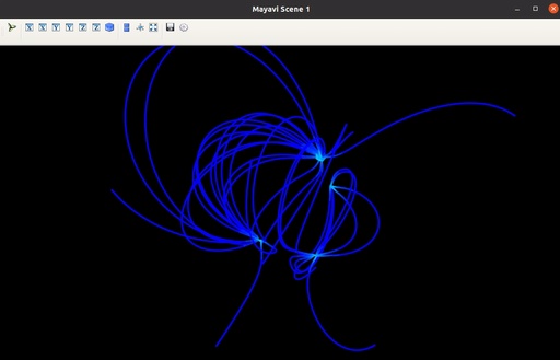
3-D Electric Field lines with Mayavi

In previous chapter I’ve already shown, how to draw continuous electric field lines with Matplotlib. But this was 2-D case. In many scientific applications, it is necessary to plot 3-dimensional field lines, and I will show how to do it with Mayavi

In is important to remember, that, despite high graphical quality of the plot, Mayavi is not very serious scientific tool and should be used with great caution.

Calculating Electric field

I already describe, how to calculate electric field die to point charges. But in all previous calculations I do use meshgrid coordinate system. Mayavi can only work with mgrid coordinate system of NumPy. Therefore we need to create domain and calculate everything is mgrid coordinate system

Because we want to see Electric field lines around charges – our domain is a bit bigger than the space for the charges. Our charges can located in the space from -1 to 1, while all domain is calculation from -3 to 3 to have some space for electric lines around these charges.


import numpy as np
from mayavi import mlab

# Domain size
s = -3.0
e = 3.0
#Step of calculations
d = 0.1
#Number of charges
NQ = 4

#Domain in mgrid coordinate system
X, Y, Z = np.mgrid[s:e:d, s:e:d, s:e:d]
#Random charges
Q = np.random.uniform(low=-1.0, high=1.0, size=(NQ, 4))

#Change charges to + and -1 only
Q[:, 3] /= np.absolute(Q[:, 3])

# Initializing array for Electric field components
Ex = np.zeros_like(X)
Ey = np.zeros_like(Y)
Ez = np.zeros_like(Z)

After initializing our domain and random charges, we can calculate electric field.

Again I do calculate squared distance first and then apply power of 1.5 to have r³ at the beginning of calculations.


for q in Q:
    r32 = ((X - q[0]) ** 2 + (Y - q[1]) ** 2 + (Z - q[2]) ** 2) ** (3 / 2)
    Ex = Ex + (q[3] * (X - q[0])) / r32
    Ey = Ey + (q[3] * (Y - q[1])) / r32
    Ez = Ez + (q[3] * (Z - q[2])) / r32

Plotting Field Lines with Mayavi

To use Mayavi plotting sistem, it is necessary to create figure first. When the image will be ready, it is possible to save it to file, or display it with function show()


mlab.figure(bgcolor=(0, 0, 0))

mlab.show()

Drawing spheres with Mayavi

At the first step I will show the position of charges and will colour them according to their charges with function points3d().


mlab.points3d(Q[:, 0], Q[:, 1], Q[:, 2], Q[:, 3], scale_factor=0.4)

For this function it is necessary to supply array of X coordinates of all spheres for displaying, then Y and Z coordinates, then optionally sizes of spheres and then optionally some parameters. Colours and sizes will be related. If you want to make size and colour independently, you should call points3d() for every charge.

Field lines

To plot streamlines for Electric Field it is necessary to calculate them with function flow() for every charge. This function need to know the coordinate grid and electric field at these coordinates. Also it is necessary to give all parameters about calculating of these streamlines, like position of starting points, direction of integration, amount of starting points, displaying or nor start points, the configuration of starting point around every charge (sphere in this case) and the width of displayed lines


lines = []
for q in Q:
    l = mlab.flow(X, Y, Z,
                   Ex, Ey, Ez,
                   integration_direction='both',
                   seedtype='sphere',
                   seed_scale=0.5,
                   seed_visible=Fasle,
                   seed_resolution=6,
                   line_width=1.0,
                   )
    lines.append(fl)

Also, it will be very useful to specify the position of starting point spheres – all starting points will be located on spheres around charges. Unfortunately, the Mayavi documentation is not good enough to find out how to do it and it is necessary to check source codes to understand these details.


    l.seed.widget.center = q[0:3]

It is also important to specify initial step for integration and the maximal length of each streamline


    l.stream_tracer.initial_integration_step = 0.1
    l.stream_tracer.maximum_propagation = 50.0

Mayavi errors.

Also it is important to mention, that Mayavi do not show every field line according to initial settings, and sometimes it is necessary to move a bit sphere with initial points to force it to show all lines.

Full code of Field liens with Mayavi


import numpy as np
from mayavi import mlab

s = -3.0
e = 3.0
d = 0.1
NQ = 4

X, Y, Z = np.mgrid[s:e:d, s:e:d, s:e:d]
Q = np.random.uniform(low=-1.0, high=1.0, size=(NQ, 4))

Q[:, 3] /= np.absolute(Q[:, 3])

Ex = np.zeros_like(X)
Ey = np.zeros_like(Y)
Ez = np.zeros_like(Z)


for q in Q:
    r32 = ((X - q[0]) ** 2 + (Y - q[1]) ** 2 + (Z - q[2]) ** 2) ** (3 / 2)
    Ex = Ex + (q[3] * (X - q[0])) / r32
    Ey = Ey + (q[3] * (Y - q[1])) / r32
    Ez = Ez + (q[3] * (Z - q[2])) / r32

mlab.figure(bgcolor=(0, 0, 0))

b.points3d(Q[:, 0], Q[:, 1], Q[:, 2], Q[:, 3], scale_factor=0.4)

lines = []
for q in Q:
    l = mlab.flow(X, Y, Z,
                   Ex, Ey, Ez,
                   integration_direction='both',
                   seedtype='sphere',
                   seed_scale=0.5,
                   seed_visible=Fasle,
                   seed_resolution=6,
                   line_width=1.0,
                   )
    l.seed.widget.center = q[0:3]
    l.stream_tracer.initial_integration_step = 0.1
    l.stream_tracer.maximum_propagation = 50.0
    lines.append(fl)

mlab.show()
mlab.points3d(Q[:, 0], Q[:, 1], Q[:, 2], Q[:, 3], scale_factor=0.4)

lines = []
for q in Q:
    l = mlab.flow(X, Y, Z,
                   Ex, Ey, Ez,
                   integration_direction='both',
                   seedtype='sphere',
                   seed_scale=0.5,
                   seed_visible=Fasle,
                   seed_resolution=6,
                   line_width=1.0,
                   )
    l.seed.widget.center = q[0:3]
    l.stream_tracer.initial_integration_step = 0.1
    l.stream_tracer.maximum_propagation = 50.0
    lines.append(fl)

mlab.show()