How to draw continuous Electric field lines
In the previous tutorials here and here, I’ve plot electrostatic lines not very correctly. The standard Matplotlib tools do not obey the main properties of electric field lines: These lines should start and finish on some charges (or go out of the area of analysis – out of the screen).
To solve this problem, it is necessary to use more specific graphics library like Mayavi, or calculate manually every electric line with integration routine in SciPy, or even write your own integration routine.
Fortunately, during the preparation of this manual, Matplotlib function streamplot was upgraded and now it is allowing to plot continuous field lines.
Upgrading Matplotlib
First of all, it is necessary to upgrade pip and then Matplotlib
python -m pip install -U pip
python -m pip install -U matplotlib
You can check your current Matplotlib version by command pip show matplotlib and it should be not older than 3.6.0 now.
Switch to continuous lines in streamplot
 continuous lines with Matplotlib."
title="Eplot with continuous lines.">
continuous lines with Matplotlib."
title="Eplot with continuous lines.">
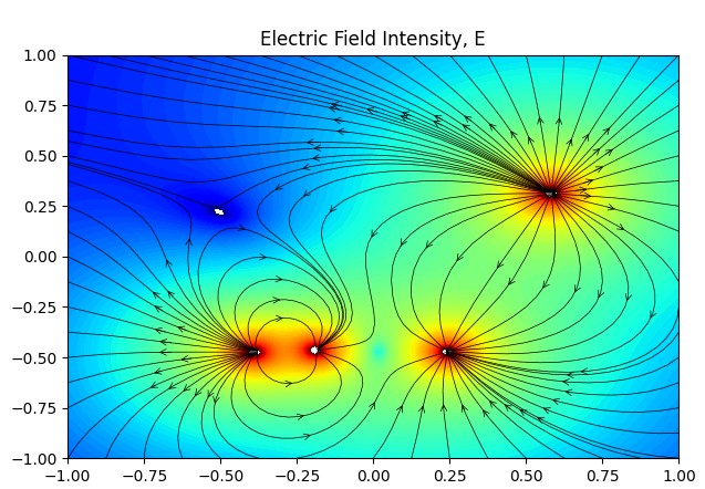
Electric Intensity Field E, calculated for 4 randomly placed charges with continuous lines with Matplotlib.
Original image: 637 x 442
To make all lines calculated properly, just add option broken_streamlines=False to the command streamplot and it will fix the problem
    ax.streamplot(D['X'], D['Y'], D['Ex'], D['Ey'], color='black', linewidth=0.5,
                  density=P['line_density'], arrowstyle='->', arrowsize=1.0,
                  broken_streamlines=False)
For more details about this modifications, please see our video:
And the full code is:
import numpy as np
import matplotlib.pyplot as plt
from matplotlib.widgets import Slider, CheckButtons, RadioButtons

def addPointCharge2D(V, Ex, Ey, X, Y, q):
    r2 = ((X - q[0]) ** 2 + (Y - q[1]) ** 2) ** (3 / 2)
    Ex += q[2] * (X - q[0]) / r2  # Electric field (x)
    Ey += q[2] * (Y - q[1]) / r2  # Electric field (y)
    V += q[2] / r2 ** (1 / 3.)
    return V, Ex, Ey


def ElectricField(E, Ex, Ey, V, X, Y, Q):
    Ex *= 0
    Ey *= 0
    V *= 0
    for q in Q:
        addPointCharge2D(V, Ex, Ey, X, Y, q)
    E[:] = np.log((Ex ** 2 + Ey ** 2)) * 0.5
    return E, Ex, Ey, V


xrange = [-1., 1.]   # left and right coordinates of square domain (x==y)
step = 40            # Number of cells in the domain in any axis
qrange = [-10., 10.] # max and min values for charge
NQ = 4               # Number of charges

P = {}  # plot description
P['plt_type'] = ['Position', 'Field', 'Lines']  # type of shown information
P['plt_active'] = [True, True, True]            # Show or not switches
P['ColorBar'] = None                            # initial colorbar
P['field_type'] = ['V', 'E']                    # available field for plotting
P['VE'] = False                                 # show vector field
P['levelE'] = np.linspace(-1, 10, 100)          # range for Efield colorbar
P['levelV'] = np.linspace(-150, 150, 100)       # range for Vfield colorbar
P['Qactive'] = 0                                # Current active charge
P['line_density_range'] = [0.1, 2.0]            # Range of possible line densities
P['line_density'] = 0.4                         # current line density

xlist = np.linspace(xrange[0], xrange[1], step)
ylist = np.linspace(xrange[0], xrange[1], step)
qmin = [xrange[0], xrange[0], qrange[0]]
qmax = [xrange[1], xrange[1], qrange[1]]

D = {}  # domain description
D['X'], D['Y'] = np.meshgrid(xlist, ylist)
D['Ex'] = np.zeros_like(D['X'])
D['Ey'] = np.zeros_like(D['X'])
D['V'] = np.zeros_like(D['X'])
D['E'] = np.zeros_like(D['X'])
D['Q'] = np.random.uniform(low=qmin, high=qmax, size=(NQ, 3))

ElectricField(**D)


############ INITIAL PLOT

def el_plot(P, D):
    P['ax'].clear()

    if P['plt_active'][0]:
        # Position
        P['ax'].scatter(D['Q'][:, 0], D['Q'][:, 1], c=np.where(D['Q'][:, 2] < 0, 'b', 'r'))
        for i, txt in enumerate(D['Q']):
            P['ax'].annotate(f'({i + 1}):{txt[2]:.1f}', xy=(D['Q'][i, 0], D['Q'][i, 1]),
                             xytext=(D['Q'][i, 0] + 0.02, D['Q'][i, 1] + 0.02),
                             color='black', fontsize='12')
    if P['plt_active'][1]:
        # Field
        if P['VE']:
            P['ax'].set_title("Electric Field Intensity, E")
            cp = P['ax'].contourf(D['X'], D['Y'], D['E'], levels=P['levelE'], cmap='jet')
        else:
            P['ax'].set_title("Electric Potential energy, V")
            cp = P['ax'].contourf(D['X'], D['Y'], D['V'], levels=P['levelV'], cmap='seismic')
        if P['ColorBar']:
            P['ColorBar'].remove()
        P['ColorBar'] = P['fig'].colorbar(cp, ax=P['ax'])

    if P['plt_active'][2]:
        # Lines
        P['ax'].streamplot(D['X'], D['Y'], D['Ex'], D['Ey'], color='black', linewidth=0.5,
                           density=P['line_density'], arrowstyle='->', arrowsize=1.0,
                           broken_streamlines=False)

    plt.draw()
    return None


P['fig'], P['ax'] = plt.subplots(figsize=(6, 5))

plt.subplots_adjust(left=0.20, bottom=0.35)
plt.xlim(xrange[0], xrange[1])
plt.ylim(xrange[0], xrange[1])

el_plot(P, D)

####################### CONTROL
####################### SLIDERS- X, Y, Q, line density

ax_x = plt.axes([0.20, 0.25, 0.55, 0.05])
ax_y = plt.axes([0.07, 0.35, 0.05, 0.53])
ax_q = plt.axes([0.20, 0.20, 0.55, 0.05])
ax_d = plt.axes([0.20, 0.15, 0.55, 0.05])

s_x = Slider(ax_x, 'x', qmin[0], qmax[0], valinit=D['Q'][P['Qactive']][0])
s_x.vline._linewidth = 0

s_y = Slider(ax_y, 'y', qmin[1], qmax[1], valinit=D['Q'][P['Qactive']][1],
             orientation="vertical")
s_y.hline._linewidth = 0

s_q = Slider(ax_q, 'q', qmin[2], qmax[2], valinit=D['Q'][P['Qactive']][2])
s_q.vline._linewidth = 0

s_d = Slider(ax_d, 'l', P['line_density_range'][0], P['line_density_range'][1],
             valinit=P['line_density'])
s_d.vline._linewidth = 0


def slider_update(val, P, D):
    q = D['Q'][P['Qactive']]

    q[0] = s_x.val
    q[1] = s_y.val
    q[2] = s_q.val
    P['line_density'] = s_d.val

    # recalculation
    ElectricField(**D)

    # output
    el_plot(P, D)


s_x.on_changed(lambda new_val: slider_update(new_val, P, D))
s_y.on_changed(lambda new_val: slider_update(new_val, P, D))
s_q.on_changed(lambda new_val: slider_update(new_val, P, D))
s_d.on_changed(lambda new_val: slider_update(new_val, P, D))

####################### CheckButton - Q, Field, Lines selector

ax_qfl = plt.axes([0.03, 0.17, 0.13, 0.13])

chxbox = CheckButtons(ax_qfl, P['plt_type'], P['plt_active'])


def qfl_select(label, P, D):
    # change clicked checkbutton
    index = P['plt_type'].index(label)
    P['plt_active'][index] = not P['plt_active'][index]

    # output
    el_plot(P, D)


chxbox.on_clicked(lambda new_select: qfl_select(new_select, P, D))

####################### RadioButton - E/V selector

ax_ev = plt.axes([0.85, 0.20, 0.10, 0.10])  # left, bottom, width, height values
rbutton1 = RadioButtons(ax_ev, P['field_type'])


def ev_select(label, P, D):
    # swap clicked rbutton
    P['VE'] = not P['VE']

    # output
    el_plot(P, D)


rbutton1.on_clicked(lambda new_select: ev_select(new_select, P, D))

####################### RadioButton - Q selector

ax_qs = plt.axes([0.01, 0.40, 0.06, 0.03 * NQ])  # left, bottom, width, height values
rbutton2 = RadioButtons(ax_qs, range(1, NQ + 1), active=P['Qactive'])


def q_select(label, P, D):
    P['Qactive'] = int(label) - 1
    q = D['Q'][P['Qactive']]

    s_x.eventson = False
    s_y.eventson = False
    s_q.eventson = False
    s_x.set_val(q[0])
    s_y.set_val(q[1])
    s_q.set_val(q[2])
    s_x.eventson = True
    s_y.eventson = True
    s_q.eventson = True

rbutton2.on_clicked(lambda new_select: q_select(new_select, P, D))

plt.show()
Published: 2022-09-26 21:46:15
Updated: 2022-09-27 19:48:58