My Coding > Software > R > Regression analysis > Linear regression analysis with R

Linear regression analysis with R (Page: 2)

Go to Page:

DPLYR: Data checking and preparation;
Linear regression model;

Our data is cleaned and ready for analysis. We will create Linear regression model with R.

COR() - correlation between data

First of all we can check, is there are any correlation between these two data with function cor()


> cor(air$Ozone, air$Wind)
[1] -0.6015465

And yes, we have negative relation of about -0.6, which mean, that when wind is increasing, the amount of ozone is decreasing.

Sign - mean about negative correlation. When one value increase, another value decreasing. Also 0.6 – mean moderate correlation. 0 – means these values are not related at all, and 1 – means these data are perfectly related.

Plot linear model between two datasets

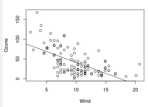
First of all we will plot this dataset with function plot(). Then can fit linear model with function lm() between these two datasets and then plot this line with abline() function


> plot(Ozone~Wind, air)
> oz_wi <- lm(Ozone~Wind, air)
> abline(oz_wi)
> oz_wi

Call:
lm(formula = Ozone ~ Wind, data = air)

Coefficients:
(Intercept)         Wind
     96.873       -5.551

After this we will have the following plot:

Linear relation beween Ozone and Wind
Plot of linear relation between Ozone concentration and Wind speed.

Statistics about our relations

Now it is time to check the statistical information about our model. For this it we need to use summary() from our linear model


> OW_summary <- summary(oz_wi)
> OW_summary

Call:
lm(formula = Ozone ~ Wind, data = air)

Residuals:
    Min      1Q  Median      3Q     Max
-51.572 -18.854  -4.868  15.234  90.000

Coefficients:
            Estimate Std. Error t value Pr(>|t|)
(Intercept)  96.8729     7.2387   13.38  < 2e-16 ***
Wind         -5.5509     0.6904   -8.04 9.27e-13 ***
---
Signif. codes:  0 ‘***’ 0.001 ‘**’ 0.01 ‘*’ 0.05 ‘.’ 0.1 ‘ ’ 1

Residual standard error: 26.47 on 114 degrees of freedom
Multiple R-squared:  0.3619,    Adjusted R-squared:  0.3563
F-statistic: 64.64 on 1 and 114 DF,  p-value: 9.272e-13

It is possible to see what kind of variables are exists in this information for individual call


> names(oz_wi)
 [1] "coefficients"  "residuals"     "effects"       "rank"          "fitted.values"
 [6] "assign"        "qr"            "df.residual"   "xlevels"       "call"
[11] "terms"         "model"

Prediction from linear model

If we satisfied with this model, we can make some predictions on the basis of this model. For this we will create data_frame with Wind vector with points of interest and apply our model to dots from this vector with function predict().


> wind_data <- data.frame(Wind = c(0, 5, 10, 15, 20, 22))
> wind_data["ozone_prediction"] <- predict(oz_wi, wind_data)
> wind_data
  Wind ozone_prediction
1    0         96.87289
2    5         69.11828
3   10         41.36367
4   15         13.60905
5   20        -14.14556
6   22        -25.24741

Go to Page: 1; 2;

Published: 2021-11-17 03:26:50
Updated: 2021-11-17 04:12:27

Last 10 artitles