Integrating 3D electric field lines with SciPy

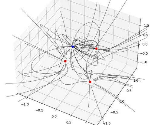
In the previous chapters I’ve describe how to calculate and plot Electric Field Lines for 2 dimensional case with ODE from SciPy. In this tutorial I will show, how you can easily swat these calculations to the 3D case.

NOTE! It is important to understand, that 3D case will use seriously more computer memory and will be much slower as well. Therefore, please pay attention for selection of the domain and grid sizes.

Essential modification from 2D to 3D conversion

Previously, all starting points were evenly distributed around point charge in the 2D space. In 3D space it is pretty difficult evenly distribute starting points around the charge. It is very difficult mathematical task about even distributing objects on the sphere. Therefore I will place these starting point randomly.

In total we will take 15 points around each sphere. Also domain will be smaller – from -2 to 2 and step-size will be 0.05. I will place 4 random charges and will make all charges +1 or -1. Again, physically, charges will be located in the space from -1 to +1


n_sphere = 15
s, e, d = -2, 2, 0.05
X, Y, Z = np.mgrid[s:e:d, s:e:d, s:e:d]
NQ = 4
Q = np.random.uniform(low=-1, high=1, size=(NQ,4))
Q[:,3] /= np.abs(Q[:,3]) # make charge +1 or -1

Electric field will be calculated for 3 dimensions. And respectively, it should be interpolated on 3D grid as well


Ex = 0*X
Ey = 0*Y
Ez = 0*Z

for q in Q:
    r2 = (X - q[0])**2 + (Y - q[1])**2 + (Z - q[2])**2
    Ex += q[3]*(X - q[0]) / r2**(3/2)
    Ey += q[3]*(Y - q[1]) / r2**(3/2)
    Ez += q[3]*(Z - q[2]) / r2**(3/2)

Exi = RGI((X[:, 0, 0], Y[0, :, 0], Z[0, 0, :]), Ex, method='linear')
Eyi = RGI((X[:, 0, 0], Y[0, :, 0], Z[0, 0, :]), Ey, method='linear')
Ezi = RGI((X[:, 0, 0], Y[0, :, 0], Z[0, 0, :]), Ez, method='linear')


def IL3(t, coord):
    global abort
    xi = coord[0]
    yi = coord[1]
    zi = coord[2]
    try:
        ex = Exi([xi, yi, zi])[0]
        ey = Eyi([xi, yi, zi])[0]
        ez = Ezi([xi, yi, zi])[0]
    except:
        abort = True
        return [0, 0, 0]
    return [ex, ey, ez]

Starting points for electric field lines

It is very difficult to distribute evenly objects on the sphere and this is not a goal for this lesson. Therefore I will do simplest distribution of the starting points on the sphere – random distribution.

I will Do select randomly angled PHI and TETA and then use them as a random spherical coordinated for the starting points.


    for i in range(n_sphere):
        phi = random.uniform(-np.pi, np.pi)
        tet = random.uniform(-np.pi, np.pi)
        lx = [q[0] + np.sin(phi) * np.cos(tet) * Rsphere]
        ly = [q[1] + np.sin(phi) * np.sin(tet) * Rsphere]
        lz = [q[2] + np.cos(phi) * Rsphere]

That it. Everything is converted, The minor leftovers, how to build 3D plot – you can find in the video about 3D electric Field Lines, or check the full working script below.

Full script


import numpy as np
import matplotlib.pyplot as plt
from scipy.integrate import ode
from scipy.interpolate import RegularGridInterpolator as RGI
import random

integrmodel = 'vode' # 'lsoda', 'dopri5', 'dop853'
max_step = 2000
step_size = 0.01
n_sphere = 15
Rsphere = 0.15
s, e, d = -2, 2, 0.05
Rsphere2 = Rsphere ** 2

X, Y, Z = np.mgrid[s:e:d, s:e:d, s:e:d]
NQ = 4
Q = np.random.uniform(low=-1, high=1, size=(NQ,4))
Q[:,3] /= np.abs(Q[:,3])
Ex = 0*X
Ey = 0*Y
Ez = 0*Z

for q in Q:
    r2 = (X - q[0])**2 + (Y - q[1])**2 + (Z - q[2])**2
    Ex += q[3]*(X - q[0]) / r2**(3/2)
    Ey += q[3]*(Y - q[1]) / r2**(3/2)
    Ez += q[3]*(Z - q[2]) / r2**(3/2)

Exi = RGI((X[:, 0, 0], Y[0, :, 0], Z[0, 0, :]), Ex, method='linear')
Eyi = RGI((X[:, 0, 0], Y[0, :, 0], Z[0, 0, :]), Ey, method='linear')
Ezi = RGI((X[:, 0, 0], Y[0, :, 0], Z[0, 0, :]), Ez, method='linear')

def IL3(t, coord):
    global abort
    xi = coord[0]
    yi = coord[1]
    zi = coord[2]
    try:
        ex = Exi([xi, yi, zi])[0]
        ey = Eyi([xi, yi, zi])[0]
        ez = Ezi([xi, yi, zi])[0]
    except:
        abort = True
        return [0, 0, 0]
    return [ex, ey, ez]

ax = plt.figure().add_subplot(projection='3d')

for q in Q:
    dt = step_size
    if q[3] < 0:
        dt *= -1
    for i in range(n_sphere):
        phi = random.uniform(-np.pi, np.pi)
        tet = random.uniform(-np.pi, np.pi)
        lx = [q[0] + np.sin(phi) * np.cos(tet) * Rsphere]
        ly = [q[1] + np.sin(phi) * np.sin(tet) * Rsphere]
        lz = [q[2] + np.cos(phi) * Rsphere]

        r = ode(IL3)
        r.set_integrator(integrmodel)

        r.set_initial_value([lx[0], ly[0], lz[0]], 0)
        step = 0
        abort = False

        while r.successful():
            step += 1
            r.integrate(r.t+dt)
            x, y, z = r.y[0], r.y[1], r.y[2]

            lx.append(x)
            ly.append(y)
            lz.append(z)

            go_out = False
            for qf in Q:
                if (x - qf[0])**2 + (y - qf[1])**2 + (z - qf[2])**2 < Rsphere2:
                    go_out = True
            if go_out:
                break

            if s >= x or e <= x or s >= y or e <= y or  s >= z or e <= z:
                break
            if step >= max_step:
                break
            if abort is True:
                abort = False
                break

        if step >= max_step:
            plt.plot(lx, ly, lz, 'r', lw=0.5)
        else:
            plt.plot(lx, ly, lz, 'k', lw=0.5)

for q in Q:
    if q[3] > 0:
        plt.plot(q[0], q[1], q[2], 'ro')
    else:
        plt.plot(q[0], q[1], q[2], 'bo')

ax.set_xlim(s, e)
ax.set_ylim(s, e)
ax.set_zlim(s, e)

plt.show()

Integrating 3D electric field lines with SciPy

Essential modification from 2D to 3D conversion

Starting points for electric field lines

Full script

Last 10 artitles

9 popular artitles