ctree clustering in R

Before start of any analysis we need to check our dataset as it described here, in the section of the data Data Preparing for Cluster analysis

In this stady we will use ctree library


> library(dplyr)
> library(party)

Training and test model

When we have a lot of data, it is easier to select randomly test set by specifying the amount of percent of data in the and training sets. From my previous experience, i’ve find out, that 5% for test set is a good enough for many kind of statistical analysis, but we will try to use 90% of data for training, just to make test set twice as big.


 iris_train <- iris %>% sample_frac(0.90)
> iris_test <- iris %>% setdiff(iris_train)

As a result, it will be 135 observations in the train set and only 14 observations in the test set.

Decision tree ctree

Calculate decision tree

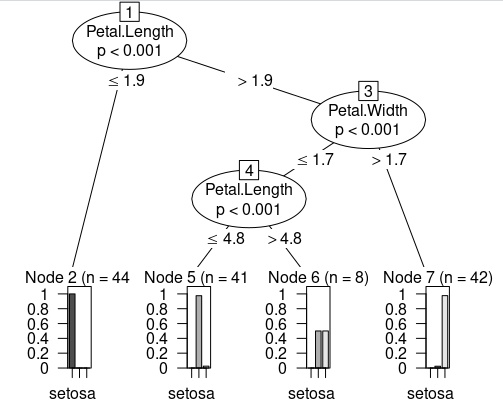
We will calculate decision tree (ctree())of relation of Species to Petal length and Petal width of irises. And then we will draw the decision tree (plot())


> iris_tree <- ctree(Species~Petal.Length + Petal.Width, data = iris_train)
> plot(iris_tree)

After this code we will have this tree

Clustering decision tree build with <b>ctree()</b> — **ctree Decision tree**
Clustering decision tree build with **ctree()**

This tree show you P-value for each decision. As you can see from this plot, only Node 6 with Petal.Length > 4.8 and Petal.Width <= 1.7 cause bad clusterings with equal amount of versicolor and virginica

Predict with decision tree

We can use this decision tree to predict our test set. We will use our calculated decision tree iris_tree to apply it towards iris_test set with function predict() and we will calculate probability of each variant type = "prob” and also will ask about classification according to these probabilities vector


> iris_test["predict"] <- predict(iris_tree, iris_test)
> iris_test
   Sepal.Length Sepal.Width Petal.Length Petal.Width    Species    predict
1           4.9         3.1          1.5         0.1     setosa     setosa
2           5.1         3.5          1.4         0.3     setosa     setosa
3           5.7         3.8          1.7         0.3     setosa     setosa
4           5.4         3.4          1.7         0.2     setosa     setosa
5           5.5         3.5          1.3         0.2     setosa     setosa
6           5.0         3.5          1.3         0.3     setosa     setosa
7           7.0         3.2          4.7         1.4 versicolor versicolor
8           6.4         3.2          4.5         1.5 versicolor versicolor
9           4.9         2.4          3.3         1.0 versicolor versicolor
10          5.0         2.0          3.5         1.0 versicolor versicolor
11          5.8         2.7          3.9         1.2 versicolor versicolor
12          7.7         2.8          6.7         2.0  virginica  virginica
13          7.4         2.8          6.1         1.9  virginica  virginica
14          6.4         3.1          5.5         1.8  virginica  virginica

At this time this clustering process give perfect result. This is amazing, and now lets’ have a look at the probability of this decision


> predict(iris_tree, iris_test, type = "prob")
[[1]]
[1] 1 0 0
[[2]]
[1] 1 0 0
[[3]]
[1] 1 0 0
[[4]]
[1] 1 0 0
[[5]]
[1] 1 0 0
[[6]]
[1] 1 0 0
[[7]]
[1] 0.00000000 0.97560976 0.02439024
[[8]]
[1] 0.00000000 0.97560976 0.02439024
[[9]]
[1] 0.00000000 0.97560976 0.02439024
[[10]]
[1] 0.00000000 0.97560976 0.02439024
[[11]]
[1] 0.00000000 0.97560976 0.02439024
[[12]]
[1] 0.00000000 0.02380952 0.97619048
[[13]]
[1] 0.00000000 0.02380952 0.97619048
[[14]]
[1] 0.00000000 0.02380952 0.97619048

It is possible to see, that the main choice always have pretty high probability.

Published: 2021-11-17 13:49:30