Spinning Earth animation with Python
In this tutorial, I will show how to make a photorealistic animation of the spinning Earth with only about 20 lines of Python code. We will not use any 3D engine or special graphics library. Everything is done with NumPy arrays and a little bit of geometry, and the Pillow library (PIL) is used only to load the picture and save the result as an animated GIF.
The main idea is very simple. We take a flat map of the Earth and wrap it around a sphere. For every pixel of our final picture, we find which point of the sphere we can see there, then which place on the map corresponds to this point, and finally how brightly this place is lit by the Sun. Real 3D graphics works in a very similar way, but here we will do everything by hand, so you can see every step.
Loading the Earth map
First of all, we will load numpy for calculations, urllib and io for downloading the picture, and PIL for working with images.
import numpy as np, urllib.request, io
from PIL import Image
Next step - we need a map of the Earth. The three.js project on GitHub has very nice free textures of planets, and we will take one of them. This map is made in the so-called equirectangular projection: longitude goes from -180° on the left edge to +180° on the right edge, and latitude goes from +90° (North Pole) at the top to -90° (South Pole) at the bottom. Every pixel is the same step in angle, and this makes the conversion from the sphere to the map very easy.
url = "https://raw.githubusercontent.com/mrdoob/three.js/dev/examples/textures/planets/earth_atmos_2048.jpg"
tex = np.asarray(Image.open(io.BytesIO(urllib.request.urlopen(url).read())).convert("RGB")) / 255
H, W = tex.shape[:2]
This line is quite long, so let's read it from the inside. urlopen(url).read() downloads the file as a set of bytes. io.BytesIO makes a file-like object in memory from these bytes, so we do not need to save anything on the disk. Image.open opens it as a picture, and convert("RGB") makes sure that we have exactly three colour channels.
Then np.asarray turns the picture into a NumPy array with the shape (1024, 2048, 3), and the division by 255 changes colour values from 0..255 to 0..1. This range is very convenient, because later we will multiply colours by the brightness of the sunlight. H and W are the height and width of the map in pixels.
Building the screen
Now we need to create our screen. N = 400 means that the final picture will be 400×400 pixels.
N = 400                                              # picture size in pixels
y, x = np.mgrid[1:-1:N * 1j, -1:1:N * 1j]            # screen, -1..1, north up
np.mgrid creates two 2D arrays with the x and y coordinates of every pixel. There is a small trick here: when the step is written as an imaginary number N * 1j, NumPy understands it not as a step, but as a number of points, including both ends. So we get exactly 400 values from -1 to 1.
Please note that y goes from 1 to -1. This is because rows in a picture go from top to bottom, and we want to see the North Pole at the top.
Which pixels show the Earth
The Earth on our screen will be a circle with radius 1 in the centre of the picture. To find all pixels inside this circle, we use the same check as in my tutorial about the Monte-Carlo calculation of the sphere volume.
inside = x**2 + y**2 <= 1inside is an array of True and False values, and later we will use it to paint everything outside the Earth black.
From the screen to the sphere
This is a very important step! Every point on the surface of a sphere with radius 1 follows the equation x2 + y2 + z2 = 1. We look at the Earth along the z axis, so for every pixel we already know x and y, and we can easily find z. The positive root gives the point on the side facing us, and the negative root would give the back side, which we cannot see anyway.
z = np.sqrt(np.clip(1 - x**2 - y**2, 0, None)) # point on the sphere facing usOutside the circle, 1 - x2 - y2 is negative, and the square root of a negative number gives NaN with a warning. np.clip simply replaces all negative values with 0. In fact, this is the so-called orthographic projection - the view of the Earth from a very large distance, as if from deep space.
Sunlight
Now let's switch on the Sun! First, we define the direction to the Sun. The vector (-1, 0.3, 1) means that the light comes from the left, a little bit from the top, and from our side. We divide it by its length (np.linalg.norm) to get a vector with length 1, which we need for the next formula.
sun = np.array([-1, 0.3, 1]) / np.linalg.norm([-1, 0.3, 1])          # direction to the Sun
light = np.clip(x * sun[0] + y * sun[1] + z * sun[2], 0, 1)          # brightness = cos(angle)
For the brightness, we use Lambert's cosine law: a matte surface is as bright as the cosine of the angle between the surface normal and the direction to the light. A sphere with radius 1 has a very nice feature - the normal at the point (x, y, z) is the vector (x, y, z) itself! So the cosine is just a dot product of two vectors: x·sun[0] + y·sun[1] + z·sun[2]. Negative values mean that this part of the surface is turned away from the Sun, so this is the night side, and np.clip changes them to 0.
Please note that the light is calculated only once. The Sun does not move relative to our camera, so the Earth turns under the light, and the line between day and night stays in the same place, as it happens in reality.
Latitude and longitude
To take colours from the map, we need to know the latitude and longitude of every visible point. The Earth's axis goes along y, so for a sphere with radius 1, y is just the sine of the latitude.
lat = np.arcsin(np.clip(y, -1, 1))np.clip here is only a safety measure against small rounding errors, because arcsin does not accept values outside the range -1..1. The latitude does not change when the Earth turns around its axis, so we calculate it before the loop.
Rotation
Now we can make our animation. We will make 72 frames, and in every frame we will turn the Earth by 360°/72 = 5°.
frames = []
for k in range(72):                                  # 72 frames = one full turn
    lon = np.arctan2(x, z) - 2 * np.pi * k / 72      # Earth turns west to east
np.arctan2(x, z) gives the angle of every point around the Earth's axis: 0 in the centre of the disk, +90° on the right edge (east) and -90° on the left edge (west). I prefer arctan2 to the normal arctan, because it works correctly in all quarters and has no problems with z = 0.
To turn the Earth, we simply shift the longitude by the angle 2πk/72. The minus sign is important here: with it, the Earth turns from west to east, as the real Earth does, so continents move from left to right and new places come from the left edge.
From the sphere to the map
Next step - we convert longitude and latitude into the column u and the row v of the map.
    u = ((lon / (2 * np.pi) + 0.5) % 1 * (W - 1)).astype(int)
    v = ((0.5 - lat / np.pi) * (H - 1)).astype(int)
lon / (2π) + 0.5 changes the longitude from the range -π..π into the range 0..1. Because of the rotation, the longitude goes outside this range, and % 1 brings it back. This is how the map closes around the globe without any gaps. Then we multiply by W - 1 and convert to integers to get the column number.
For the row, the North Pole (latitude π/2) gives the top row 0, and the South Pole (latitude -π/2) gives the bottom row H - 1. astype(int) simply cuts off the fractional part, so we take the nearest pixel of the map. With a 2048-pixel map and a 400-pixel picture, this is quite enough.
Painting the frame
Now we just need to put the picture together. This one line does all the painting!
img = tex[v, u] * (0.04 + 0.96 * light)[..., None] * inside[..., None]tex[v, u] uses NumPy fancy indexing. u and v are 400×400 arrays of indices, so the result is a 400×400×3 picture, where every pixel takes its colour from the map. This is done in one operation, without any Python loops over pixels, and this is the main reason why the code is so fast.
Then we multiply the colours by the brightness. 0.04 + 0.96 * light gives 4% of ambient light, so the night side is very dark but not completely black, and 100% brightness where the Sun shines directly. [..., None] adds a third axis to the 400×400 arrays light and inside, so NumPy can multiply them by the 400×400×3 colour array (this is called broadcasting). Multiplication by inside makes all the space around the Earth black.
Saving the GIF
The last step is to save the result.
    frames.append(Image.fromarray((img * 255).astype(np.uint8)))
frames[0].save("earth.gif", save_all=True, append_images=frames[1:], duration=40, loop=0)
In every frame, we convert the colours back from 0..1 to integers 0..255 and make a PIL picture. Then the first frame saves the whole animation: save_all=True tells PIL to write many frames, and append_images gives it the rest of them. duration=40 means 40 milliseconds per frame, which is 25 frames per second, so one full turn of the Earth takes 72 × 40 = 2880 ms, about 3 seconds. loop=0 means that the animation will repeat forever.
The file is quite big, about 5 MB. If you need a smaller GIF, you can reduce N or the number of frames (do not forget to change 72 in both places).
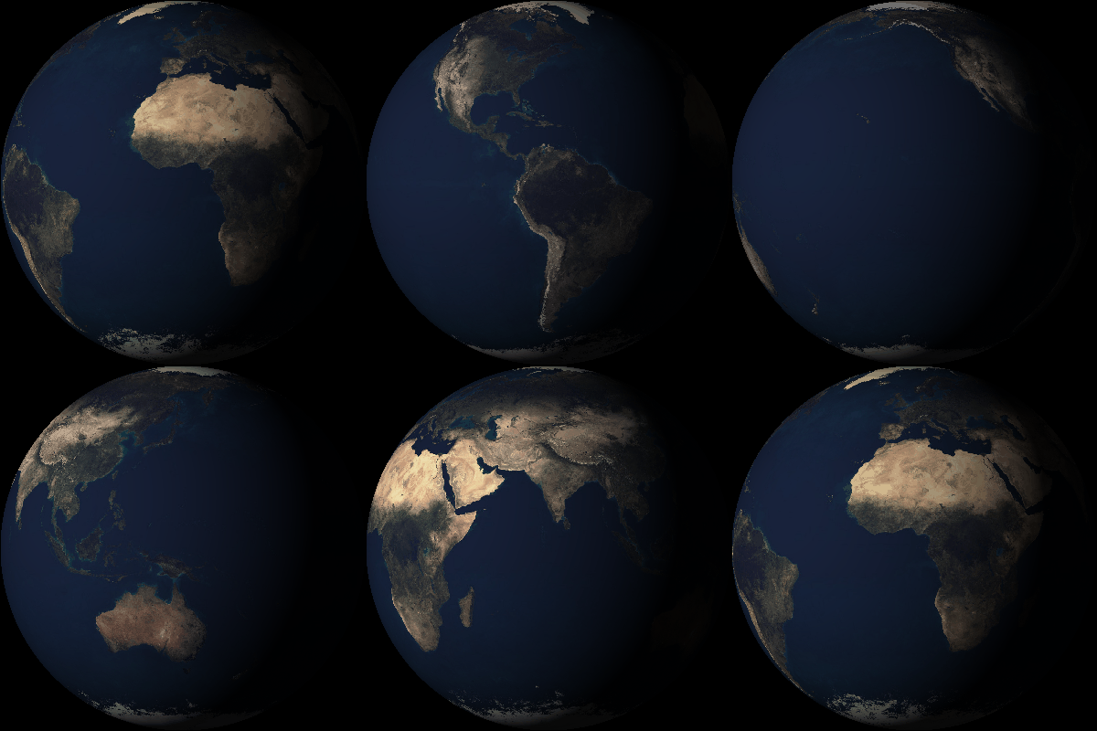
Animated GIF of the spinning Earth, made with NumPy and Pillow only. The flat map is wrapped around a sphere, lit by the Sun with Lambert's cosine law and turned by 5° in every frame.
These are absolutely amazing results for only 20 lines of code! And you can easily play with this program. Change the direction to the Sun, and you will see the Earth at a different time of day. Or change the texture: in the same three.js folder there is a map of the Moon (moon_1024.jpg), so with one changed line you can make a spinning Moon. You can even try to add the map of city lights (earth_lights_2048.png) to the night side.
Full code
For your convenience, here is the whole program in one block.
import numpy as np, urllib.request, io
from PIL import Image

url = "https://raw.githubusercontent.com/mrdoob/three.js/dev/examples/textures/planets/earth_atmos_2048.jpg"
tex = np.asarray(Image.open(io.BytesIO(urllib.request.urlopen(url).read())).convert("RGB")) / 255
H, W = tex.shape[:2]

N = 400                                              # picture size in pixels
y, x = np.mgrid[1:-1:N * 1j, -1:1:N * 1j]            # screen, -1..1, north up
inside = x**2 + y**2 <= 1
z = np.sqrt(np.clip(1 - x**2 - y**2, 0, None))       # point on the sphere facing us
sun = np.array([-1, 0.3, 1]) / np.linalg.norm([-1, 0.3, 1])          # direction to the Sun
light = np.clip(x * sun[0] + y * sun[1] + z * sun[2], 0, 1)          # brightness = cos(angle)
lat = np.arcsin(np.clip(y, -1, 1))

frames = []
for k in range(72):                                  # 72 frames = one full turn
    lon = np.arctan2(x, z) - 2 * np.pi * k / 72      # Earth turns west to east
    u = ((lon / (2 * np.pi) + 0.5) % 1 * (W - 1)).astype(int)
    v = ((0.5 - lat / np.pi) * (H - 1)).astype(int)
    img = tex[v, u] * (0.04 + 0.96 * light)[..., None] * inside[..., None]
    frames.append(Image.fromarray((img * 255).astype(np.uint8)))
frames[0].save("earth.gif", save_all=True, append_images=frames[1:], duration=40, loop=0)
Published: 2026-10-16 19:30:24