Polynomial fit with Numpy polyfit
Why we need Polynomial fit?
Suppose you have some experimental dependency Y for X, in some reasonably limited range and this function is not indefinitely periodical. In that case, you can model, or approximate it with a polynomial function with the general formula:
\[P(x) = \sum_{k=0}^{n} a_k x^k = a_n x^n + a_{n-1} x^{n-1} + a_{n-2} x^{n-2} + \ldots + a_1 x + a_0\]
Strictly speaking, every function without breaks can be modelled as a polynomial function, but the coefficient can be diverged for some of them.
In this work, we will consider good function - almost without discontinuity and only on a reasonable short interval, defined analytically. I will show how to approximate this function with a polynomial function in Numpy.
For the test, I will use the following function:
\[y = \begin{cases} x, & 0 \leq x < 1 \\ \frac{1}{x}, & 1 \le x \leq 5 \end{cases}\]
As you can see, this function is piecewise with no breaks, but its derivative, especially the second derivative, has breaks, which can be unsuitable in some cases. Therefore, we need to model it as a polynomial function.
Or, we have a set of experimental values and need to approximate them with some function for further simple calculations—in this case, polynomial approximation can also be reasonable.
To estimate the quality of this approximation we can calculate RMSD - Root Mean Square Deviation - standard value for estimating the difference between models. It can be calculated by equation:
\[\text{RMSD} = \sqrt{\frac{1}{N} \sum_{i=1}^{N} \left( y_i - \hat{y}_i \right)^2}\]
Numpy tools for polynomial fit
Numpy offers a range of different methods, which can be used for manipulations with polynomial data. The most important are: polyfit, polyval and poly1d.
Numpy polyval
The parameters are very simple numpy.polyval(p, x) - it will calculate the value of
\[p_0*x^{(N-1)} + p_1*x^{(N-2)} + ... + p_{N-2}*x + p_{N-1}\]
for every x given. Generally speaking, it is easy to calculate it without this function, but when you have the polynomial coefficient, this function is faster than a cycle.
Numpy poly1d
The poly1d is a class in NumPy that creates a polynomial object. Once you create a poly1d object, you can easily evaluate it, perform arithmetic operations, and even access its derivative or integral. Generally speaking, if you are planning to do some manipulations with polynome, it is better and more convenient to use this class. For example:
import numpy as np
# Create a polynomial object p(x) = 2x^2 + 3x + 4
p = np.poly1d([2, 3, 4])
# Evaluate at x = 5
result = p(5)  # Returns 2*(5^2) + 3*(5) + 4 = 69
# Derivative of p(x)
derivative = p.deriv() # Will have polynomial = 4x + 3
# Integral of p(x)
integral = p.integ() # Will have polynomial = 0.6667x^3 + 1.5x^2 + 4x
As you can see, this class is very useful for many manipulations of polynomial functions.
Numpy polyfit
Least squares polynomial fit. The standard basic use of this code is numpy.polyfit(x, y, deg), where X, Y - is the list of X and Y points to be fitted with the polynomial function of power deg. An example of this function usage can be found below.
Polynomial fit for the given function
Simple fit of the polynomial function
Let's consider the simple usage of the polynomial fit function in the following code. The comments in the will describe the idea of this usage.
# Import necessary libraries
import numpy as np
# Creating an array of equally distributed dots for plotting
x = np.linspace(0, 5, 100)
# Array for function values
y = np.zeros_like(x)
# Calculating function values via splitting data set with mask
mask = x >= 1
y[~mask] = x[~mask]
y[mask] = 1/x[mask]

# Using polyfit function for fitting of the polynomial function  of power 4
degree = 4
coef = np.polyfit(x, y, degree)
# printing polynomial function
print("y = ", " + ".join([f"{x:.2f}*x^{len(coef)-id-1}" for id, x in enumerate(coef)]))

# Calculation of the prediction values for the know X array
y_pred = np.polyval(coef, x)

# Calculation of the RMSD
RMSD = np.sqrt(np.mean((y - y_pred) ** 2))

# Print RMSD
print(f"{RMSD=}")
This code will print the polynomial function and RMSD: y = -0.03*x^4 + 0.35*x^3 + -1.38*x^2 + 1.93*x^1 + -0.09*x^0 and RMSD=0.059084821745851446, witch is enough for the further work.
As you can see from the code above, the general usage of this function is simple and straightforward.
To study the function and its behaviour, it is more interesting to present everything as a graph. Let's do it in the following section
Graphical representation
We do not need to make a big difference in the code, only it is necessary to add graphical output.
This is the first part of the program, almost identical to the previous code. The only difference is that one more array was created to calculate the polynomial function by dots. Ideally, these dots should be different from the experimental set to see the difference more clearly, if any.
import numpy as np
import matplotlib.pyplot as plt

x = np.linspace(0, 5, 100)
y = np.zeros_like(x)

mask = x >= 1
y[~mask] = x[~mask]
y[mask] = 1/x[mask]

initial_degree = 5
coef = np.polyfit(x, y, initial_degree)
# Calculating polynomial function by given coefficients
x_fit = np.linspace(min(x), max(x), 100)
y_fit = np.polyval(coef, x)

# Calculate RMSD
y_pred = np.polyval(coef, x)
RMSD = np.sqrt(np.mean((y - y_pred) ** 2))
When everything is calculated, we can plot these data as two graphs
# Plotting
fig, (ax1, ax2) = plt.subplots(2, 1, figsize=(8, 8))
#Experimental set and modelled polynomial line
ax1.scatter(x, y)
ax1.plot(x_fit, y_fit, label=f'power = {initial_degree}; RMSD={RMSD:.3f}', color='red')
ax1.legend()
# Coefficient of the polynomial function
ax2.plot(range(initial_degree+1), coef[::-1], marker='o')
ax2.set_xlabel('Power')
ax2.set_ylabel('Coef')
ax2.set_title('Polynomial Coef')

plt.show()
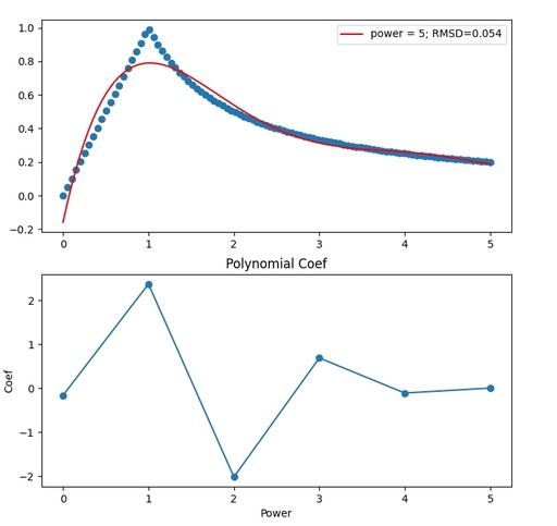
Graphical comparison of the experimental function and polynomial curve of the power 5. The coefficients of the polynomial function are given in the second plot.
Original image: 735 x 694
Interactive study of polyfit
It is possible to plot and calculate data for the different powers, but sometimes it can be ey useful to observe it in dynamics, how changing the polynomial power can affect the quality of the solution. Let's do it with matplotlib widgets.
The idea of the code will be the same, but in this case, we will calculate coefficients for all possible powers from 1 to 100 and then, with widget will plot the required polynomial function.
First of all, we need to define all functions and do not forget to include the widgets libraries. Also, if you want to use this in juputer notebook, then it is necessary to use the proper key: %matplotlib widget.
Function for calculating our target function, which we need to approximate.
#%matplotlib widget
import numpy as np
import matplotlib.pyplot as plt
from matplotlib.widgets import Slider

def my_func(x):
    y = np.zeros_like(x)
    mask = x>=1
    y[~mask] = x[~mask]
    y[mask] = 1/x[mask]
    return y
Then function for plotting our graphs
def plot_polynomial_fit(D, CF, YF, RMSD, x, y):
    # Cleaning previous view
    ax1.cla()
    ax2.cla()
    # Creating target function at dots
    ax1.scatter(x, y)
    # Creating fitted polynomial function
    ax1.plot(x, YF[D], label=f'power = {D}; RMSD={RMSD[D-1]:.3f}', color='red')
    ax1.legend()
    # Plotting of the coefficient from x^0 to x^power
    ax2.plot(range(D+1), CF[D-1][::-1], marker='o')
    ax2.set_xlabel('Power')
    ax2.set_ylabel('Coef')
    ax2.set_title('Polynomial Coef')
    #Drawing the plot
    plt.draw()
Now we need to have a function, which will handle the widget calls. This function will catch any changes in the widget scroll and call the plot function with new parameters.
def update(val, CF, YF, RMSD, x, y):
    degree = int(degree_slider.val)
    plot_polynomial_fit(degree, CF, YF, RMSD, x, y)
Now we need to prepare all the data.
# Calculate target function
x = np.linspace(0,6,100)
y = my_func(x)
# Lists for storing results for every degree
CF = []
YF = []
RMSD = []
# calculating coefficient and parameters for every degree
for degree in range(1, 101):
    CF.append( np.polyfit(x, y, degree))
    YF.append(np.polyval(CF[-1], x))
    RMSD.append(np.sqrt(np.mean((y - YF[-1]) ** 2)))
When you run your code you will have an error:
poly2.py:41: RankWarning: Polyfit may be poorly conditioned
  CF.append( np.polyfit(x, y, degree))
The warning message RankWarning: Polyfit may be poorly conditioned is triggered when using NumPy's polyfit function to fit a polynomial to data points, particularly when the degree of the polynomial is too high relative to the data provided.
Poorly conditioned means that the system of equations generated to fit the polynomial is numerically unstable, leading to large errors in the polynomial coefficients. This happens because fitting a high-degree polynomial can lead to issues with floating-point precision and large differences in the magnitude of terms in the system, which causes instability. In practice, a poorly conditioned fit implies that the polynomial may not accurately represent the underlying data and might exhibit extreme oscillations or overfitting.
Overfitting
A high-degree polynomial will try to pass through or near every data point, which may cause the curve to oscillate wildly, especially if the data is noisy or sparse.
Numerical instability
Higher-degree polynomials involve very large and very small powers of x, which can cause numerical precision problems. Small rounding errors in the coefficients can lead to large deviations in the results.
Now we can plot our results.
# Initial power for plotting
initial_degree = 3
# Create plots with fixed borders to make space for widget
fig, (ax1, ax2) = plt.subplots(2, 1)
plt.subplots_adjust(left=0.1, right=0.9, top=0.9, bottom=0.2)
#Plotting initial case
plot_polynomial_fit(initial_degree, CF, YF, RMSD, x, y)
#Location of the widget slider
ax_slider = plt.axes([0.1, 0.1, 0.8, 0.03])
degree_slider = Slider(ax_slider, 'Power', 1, 100, valinit=initial_degree, valstep=1)
# Reaction on the sliders' move
degree_slider.on_changed(lambda val: update(val, CF, YF, RMSD, x, y))
#Final plot
plt.show()
This will produce the widget:

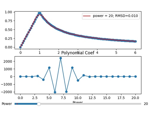
Interactive representation of the experimental function and polynomial curve with the ability to change power from 1 to 100. The coefficients of the polynomial function are given in the second plot.
Original image: 615 x 468
To check the RMSD it is possible to use a very simple piece of code:
plt.plot(RMSD)
plt.title("RMSD")
plt.show()
which will produce

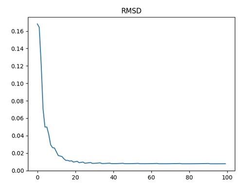
RMSD for different powers of the polynomial function
Original image: 597 x 442
As you can see, RMSD drops dramatically in the range from 1 to 15 and then starts to oscillate. This oscillation is related to the pseudo-even and odd polynomial function behaviour. It is better to stop at the maximal power of 15.
Let's plot the Maximal by module coefficients.
CFF = [ np.max(np.abs(cf)) for cf in CF ]
plt.plot(CFF)
plt.title("Maximal by module coefficients")
plt.show()
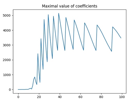
The maximal polynomial coefficient for the different polynomial powers.
Original image: 579 x 454
As you can see, up to power of 15, the coefficients are low and then that's to increase significantly, which means that it is overfitting. The oscillation of the high values means overfitting as well.
Published: 2024-10-18 19:28:49
Updated: 2024-10-19 14:46:49