How to fit line with fixed point
Very common task for many scientific fields is to find the line, which is best fitted to a given set of data. Sometimes this task is a bit more complicated, because sometimes we have some restrictions to the coefficients of this line or curve.
In this topic I will show you how to best fit the line and what to do if we have requirement to fix coefficient of this line.
I already give one way of solving this problem before, see article about Ridge regression for approximate solution of linear equation, but now I need to make some extra notices.
Task: Best line with fixed point
This is a real scientific task – find the best fitted line y=k*x+b for out data [xi, yi] with requirements that this line must go through the point (0,0).
First of all, if we have the requirement with other coordinates, we can do parallel shift of coordinate system, to move the origin of our system to this point for simplify our calculations.
If y=k*x+b cross the point (0,0) then we can find b coefficient:
0 = k*0 + b => b = 0;
Solution: Best line with fixed point
So we need to find minima of the function Σ(k*xi + b – yi)2 when b equal 0.
Solving this equation we obtain formula:
k = Σxi*yi / Σx2i
You can see short lecture about Linear regression analysis with fixed intercept
It is not much to show how to code this simple task, but I will give you some example and compare RMSD with proper best solution without any fixed coefficients.
Sample of the task for best fitted line
We will use libraries NumPy and mathplotlib.
import numpy as np
import matplotlib.pyplot as plt
Then we need to prepare task for solving, this will be random cloud of dots, with fixed random start for repeatability.
np.random.seed(0)
x = np.random.rand(50)*10
y = x * np.random.rand(50) + 1
Best fit with Numpy Polifit()
For finding best poli-line fitted to our dataset we can just call function polyfit with mentioning the order of this line (1 for linear case)
kp, bp = np.polyfit(x,y,1)
print(kp, bp)
#0.3992235424197471 0.975694629054904
Best fit with fixed 0
We can use polyfit() function as well with adding point (0, 0) with higher weight, but this is not necessary if we have exact analytical solution, according to formula k = Σxi*yi / Σx2i
k = np.sum(x*y)/np.sum(x**2)
print(k)
# 0.5436083924466607
it is possible to see some difference between 0.3992235424197471 and 0.5436083924466607
RMSD between datasets.
To find, how good our solution corresponds to the given dataset. By the definition, RMSD = √((1/n)*Σ(yi-ymean)2). We can make this calculation from scratch, or we can use some good formulas from NumPy library
We need to find RMSD not from some mean value, but difference between two datasets. So, we will use this code for doing this:
def rmsd(y1,y2):
    return np.sqrt(np.mean((y1-y2) ** 2))
where y1 and y2 - numpy arrays with Y values for the same X.
Final code with comparison of two best fits
That it. We are ready to put all code together
import numpy as np
import matplotlib.pyplot as plt

def rmsd(y1,y2):
    return np.sqrt(np.mean((y1-y2) ** 2))

np.random.seed(0)

xx = np.linspace(-1,12,2)

x = np.random.rand(50)*10
y = x * np.random.rand(50) + 1
#y = kx + b
kp, bp = np.polyfit(x,y,1)
print(kp,bp)
k = np.sum(x*y)/np.sum(x**2)
print(k)

plt.plot(x, y, 'o', c='y', label = 'data')
plt.plot(xx, kp*xx+bp, c='r', label=f'rmsd={rmsd(y, kp*x+bp):.3f}')
plt.plot(xx, k*xx, c='k', label=f'rmsd={rmsd(y, k*x):.3f}')
plt.legend(loc='upper left')
plt.show()
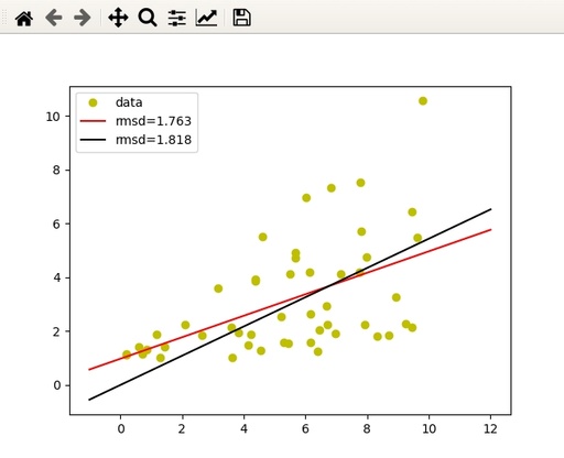
Which will give the following result:

Compare proper linear regression, calculated with polyfit() and theoretical regression with fixed intercept point.
Original image: 634 x 515
Published: 2022-07-21 23:15:09