How to calculate numerical derivative with Python

This is a simplest code for numerical calculating of a derivative of any analytical function, which you can calculate in any points.

Definition of derivatives

By definition, the derivative of function f(x) in the point x is equal [f(x+Δx) – f(x)]/Δx, when Δx is approaching to 0. Roughly speaking, the lest Δx you taking for calculations, the more accurate value of derivative you will get.

Therefore, if we have tabulated for function data eventually distributed over the X axis, then the numerical derivative in the simplest case will be f’(x_i) = (f(x_i+1)-f(x_i))/dx.

Coding for differentiation

For example I will calculate the derivative of sin(x) and then visually compare it with theoretical solution cos(x)

Including libraries

For the derivative calculations we only need NumPy library and matplotlib for graphical output.


import numpy as np
import matplotlib.pyplot as plt

Calculating of our function and derivative

Functions for calculating of function value and theoretical derivative we can take from numpy library also. For this example we will take f(x) = sin(x), then , the derivative will be f’(x) = cos(x).


def f(x):
    return np.sin(x)
def df(x):
    return np.cos(x)

Physical domain and borders

For calculation we will need to define physical size of our domain, or area of calculations.

We will take user defined s_x start of the domain and e_x end of the domain. Also we need to know number of cots or cells in this domain n_x

Border will be defines as 1 – good enough for this algorithm. And the we will store these user difined values into a compact structure x, used in all calculations.


s_x = -10.0
e_x = 10.0
n_x = 100

border = 1
x = {'b': border,
     's': 0,
     'e': n_x + 2 * border,
     'l': border,
     'r': n_x + border,
     'd': (e_x - s_x)/n_x,
    }

Calculating all values

first of all we will uniformly arrange x values in our domain with np.arange function

Then we need to prepare numpy array for numerical derivative U, calculate our function Y and theoretical derivative dY


X = np.arange(start = s_x - x['d']*x['b'],
               stop = e_x + x['d']*x['b'],
               step = x['d'])
U = np.empty_like(X)
Y = f(X)
dY = df(X)
U = derivative(U, Y, x)

Function for differentiation


def derivative(res, f, x):
    res[x['l']:x['r']] = (f[x['l']+1:x['r']+1] - f[x['l']:x['r']])/x['d']
    return res

Graphical output

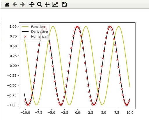
Draw everything for visual inspection. Yellow – our function. Black – theoretical derivative. Red crosses – numerically calculated derivatives.


plt.plot(X,Y, c='y', label = 'Function')
plt.plot(X,dY, c='k', label = 'Derivative')
plt.plot(X[x['l']:x['r']],U[x['l']:x['r']], 'x', c='r', label = 'Numerical')
plt.legend(loc='upper left')
plt.show()

Full code


import numpy as np
import matplotlib.pyplot as plt

# derivative calculation
def derivative(res, f, x):
    res[x['l']:x['r']] = (f[x['l']+1:x['r']+1] - f[x['l']:x['r']])/x['d']
    return res

# Our function and derivatrive for comparison
def f(x):
    return np.sin(x)
def df(x):
    return np.cos(x)

# User defined values    
s_x = -10.0
e_x = 10.0
n_x = 100

#Compact storage of domain parameters
border = 1
x = {'b': border,
     's': 0,
     'e': n_x + 2 * border,
     'l': border,
     'r': n_x + border,
     'd': (e_x - s_x)/n_x,
    }

# Arangingx values over the axis
X = np.arange(start = s_x - x['d']*x['b'],
               stop = e_x + x['d']*x['b'],
               step = x['d'])
# data structure for derivative
U = np.empty_like(X)
# clculationg of our function and theoretical derivative
Y = f(X)
dY = df(X)

# calculating of numerical derivative
U = derivative(U, Y, x)

# final graphical output
plt.plot(X,Y, c='y', label = 'Function')
plt.plot(X,dY, c='k', label = 'Derivative')
plt.plot(X[x['l']:x['r']],U[x['l']:x['r']], 'x', c='r', label = 'Numerical')
plt.legend(loc='upper left')
plt.show()