Linear regression analysis with R (Page: 1)
In statistics, linear regression is a linear approach for modelling the relationship between a scalar response and one or more explanatory variables (also known as dependent and independent variables).
Before data analysis, it is necessary to check our data, understand the format of this dataset and check for the quality, buy removing some information which is not useful for our purposes.
For this analysis I will show how to use dplyr library. First of all you need to install this library, and then when you start R or rstudio it is necessary to load this library first library(dplyr)
Overview of the dataset
Read information about dataset
Some datasets already have information about it’s content. In this case it is very usefull to use command help()
> help(airquality)
airquality              package:datasets               R Documentation
New York Air Quality Measurements
Description:
     Daily air quality measurements in New York, May to September 1973.
Usage:
     airquality

Format:
     A data frame with 154 observations on 6 variables.

       ‘[,1]’  ‘Ozone’    numeric  Ozone (ppb)
       ‘[,2]’  ‘Solar.R’  numeric  Solar R (lang)
       ‘[,3]’  ‘Wind’     numeric  Wind (mph)
       ‘[,4]’  ‘Temp’     numeric  Temperature (degrees F)
       ‘[,5]’  ‘Month’    numeric  Month (1-12)
       ‘[,6]’  ‘Day’      numeric  Day of month (1-31)
glimpse – simple overview columns
For simple in formation about available columns, it is possible to use function glimpse()
> library(dplyr)
> glimpse(airquality)
Rows: 153
Columns: 6
$ Ozone    41, 36, 12, 18, NA, 28, 23, 19, 8, NA, 7, 16, 11, 14, 18, ...
$ Solar.R  190, 118, 149, 313, NA, NA, 299, 99, 19, 194, NA, 256, 29...
$ Wind     7.4, 8.0, 12.6, 11.5, 14.3, 14.9, 8.6, 13.8, 20.1, 8.6, 6...
$ Temp     67, 72, 74, 62, 56, 66, 65, 59, 61, 69, 74, 69, 66, 68, 5...
$ Month    5, 5, 5, 5, 5, 5, 5, 5, 5, 5, 5, 5, 5, 5, 5, 5, 5, 5, 5...
$ Day      1, 2, 3, 4, 5, 6, 7, 8, 9, 10, 11, 12, 13, 14, 15, 16, 17...
Quick visualizing of the dataset
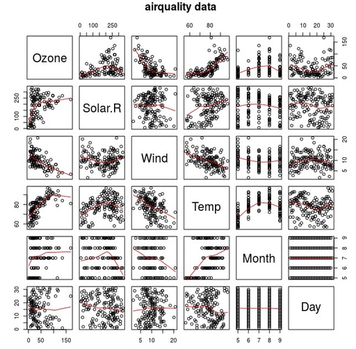
It is possible to overview these data by quickly displaying all data in the simple pair graphs
> require(graphics)
> pairs(airquality, panel = panel.smooth, main = "airquality data")
After executing these two lines you should have something like that:

Paris relation in Air quality test dataset.
Original image: 646 x 634
NA – missed data
Next step of data analysis, is to check the absence for some data in the set. And if any data is missed it will have value NA - it is necessary to understand what will you do with this data, but this is a question for future investigations. To check the presence on NA use function anyNA() to all dataset or to any of its columns
> anyNA(airquality)
[1] TRUE
> anyNA(airquality$Ozone)
[1] TRUE
> anyNA(airquality$Wind)
[1] FALSE
As you can see, that the dataset have some NA data and further analysis reveals, that Ozone column have some missed data, but Wind column is completely full
Filtering datasets
We will remove all data with NA values from our dataset. For this we will pipe %>%our dataset to a new with filter() of NA data from Ozone column
> air <- airquality %>% filter(is.na(Ozone)==FALSE)And from now we will work with new dataset air
Summary
Now, when dataset is cleaned from absent data, we can check it summary with command summary()
> summary(air$Ozone)
   Min. 1st Qu.  Median    Mean 3rd Qu.    Max.
   1.00   18.00   31.50   42.13   63.25  168.00
> summary(air$Wind)
   Min. 1st Qu.  Median    Mean 3rd Qu.    Max.
  2.300   7.400   9.700   9.862  11.500  20.700
Published: 2021-11-17 03:26:50
Updated: 2021-11-17 04:12:27