Reading FITS files with astropy
About FITS
FITS stands for Flexible Image Transport System, a standard file format widely used in astronomy for storing, transmitting, and processing scientific data, particularly images and tables.
The key components of a FITS file are Header Data Units (HDUs). Each FITS file can contain one or more HDUs, and each HDU consists of a header and optional data.
About HDU
There are two main types of HDUs:
- Primary HDU (PHDU): The primary HDU is the main header unit and contains the primary data array. The primary data array might represent an image, a spectrum, or a table, depending on the nature of the observation.
- Image HDU (Image Extension): Additional HDUs beyond the primary HDU can be used to store supplementary data. These can include images, tables, or other data types related to the primary observation. Each extension has its own header and data array.
Reading and displaying FITS file
In this article, I will show how to extract image data from the FITS file on the example of the SDO telescope.
It is possible to download this FITS file here:
| Example of FITS file SDO_20151014_cut.fits (2,263,680 b) |
| An example of the FITS file from SDO telescope, collected with 171 angstrom wavelength |
First of all, we need to load all required libraries. astropy.io - for reading FITS file and optionally astropy.visualization for improving style of image displaying.
from astropy.io import fits
from astropy.visualization import astropy_mpl_style
import numpy as np
import matplotlib.pyplot as plt
The next step is reading the file and printing the number of HDU blocks inside. FITS file should have a primary HDU block and all other blocks are optional.
From this file, we extract the header and data. Now data have an image we will analyze further. It is important to remember to close the opened file
fname = 'SDO_20151014_cut.fits'

hdus = fits.open(fname)
print(f"File `{fname}` have {len(hdus)} HDU blocks")
data = hdus[0].data
header = hdus[0].header
hdus.close()
After closing the file, we still can have access to the header and data, and the code given below should not cause any error, but it is not recommended to do this. After closing the file, only the block from the memory is available. And everything else is unavailable. As you know, some astronomical images can be too big to be read completely to the memory. Therefore, I do advise you not to use closed files, but rather extra information prior to closure.
The header has all information about an image
print(f"Header = {hdus[0].header}")This is the correct way of checking the size of the image. You can see that this is a monochrome image, which corresponds to the one-wavelength data collection. 171 Å, as you can see from the header lines WAVELNTH= 171 and WAVEUNIT= 'angstrom'.
print(f"Shape = {data.shape}")
#Shape = (833, 1347)
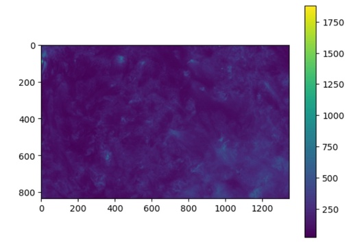
Let's display this image with the imshow function.
plt.figure()
plt.imshow(data)
plt.colorbar()
plt.show()
You should have something like this image:

The fragment of the solar surface imaged by SDO at the wavelength of 171Å, displayed with the default settings.
Original image: 887 x 619
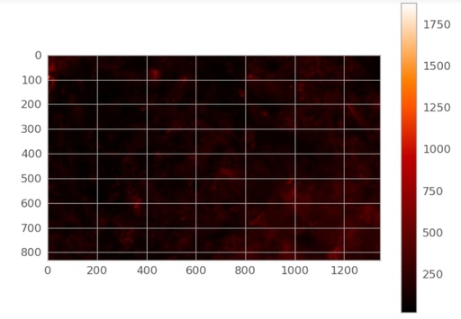
To make the image fit astronomical standards, it is a good idea to apply astropy_mpl_style from the astropy.visualization library:
plt.style.use(astropy_mpl_style)
plt.figure()
plt.imshow(data)
plt.colorbar()
plt.show()
Now you will have something like this:

The fragment of the solar surface imaged by SDO at the wavelength of 171Å, displayed with the improved astronomical standard settings following the astropy_mpl_style.
Original image: 1086 x 752
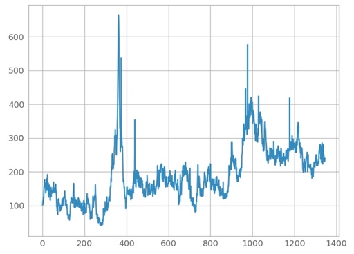
Now we can analyze the intensity along some direction, but this is not very meaningful. For example, this is a slice along x=600. This slice is not good for scientific analysis of the data but can be useful for technical or test purposes.
plt.plot(data[600,:])
plt.show()
the result will be similar to this one:

Slice of the solar image along the line x=600.
Original image: 848 x 609
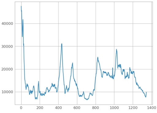
A better way to analyze some features of the image is to use the total intensity of the thin layers of the image. For example, around the area with x=100, I've noticed some bright spots and want to check them. For this, I will do a slice from 50 to 150 and make a sum along axis=0.
spot = np.sum(data[50:150, :], axis=0)
plt.plot(spot)
plt.show()
Integrated slice of the solar image for the x-axis in the range from 50 to 150.
Original image: 848 x 609
The full code at once is given below, and for test purposes, I do advise you to use Jupyter Notebook.
from astropy.io import fits
from astropy.visualization import astropy_mpl_style
import numpy as np
import matplotlib.pyplot as plt

fname = 'SDO_20151014_cut.fits'

hdus = fits.open(fname)
print(f"File `{fname}` have {len(hdus)} HDU blocks")
data = hdus[0].data
header = hdus[0].header

hdus.close()
print(f"Header = {hdus[0].header}")

print(f"shape = {data.shape}")

plt.figure()
plt.imshow(data)
plt.colorbar()
plt.show()


plt.style.use(astropy_mpl_style)
plt.figure()
plt.imshow(data)
plt.colorbar()
plt.show()

plt.plot(data[600,:])
plt.show()

spot = np.sum(data[50:150, :], axis=0)
plt.plot(spot)
plt.show()
Published: 2023-12-02 06:27:50
Updated: 2023-12-02 11:05:34