Monte-Carlo method for sphere volume calculation
In this tutorial. I will show, how to use the Monte-Carlo technique for the calculation of the volume of the n-dimensional sphere, or, so-called, n-ball. This method is great for cases when you don't know how to use equations, but you can find a way to classify your data by good or bad. For example for n-ball, we can think that you don't know the equation for the volume calculation, but can easily say if this dot stays within the sphere or outside.
So the main idea of the Monte Carlo method is to use randomly casted points and compare the filling of the test figure with the unknown figure and then do a proportional ratio of their properties.
Sphere volume
2D sphere volume
For the 2D sphere volume we use different words and call them circle surface, but generally speaking, this is the volume of this object. So, let's calculate it with the Monte Carlo technique.
First of all, we will load numpy for calculation and matplotlib for presentation.
import numpy as np
import matplotlib.pyplot as plt
Next step - we need to define the initial parameters. Square size - square, which will have a circle inside. By comparing a number of random dots within the square and circle we can say about the relations of the square and circle area. N=100 - number of random trials.
square_size = 2
radius = 1
N = 100
Now we do this Monte Carlo random experiment. to generate N random dots within the square, Then, for every tod we calculate the distance from the centre, and then if this distance is less than the standard radius, we will classify this dot as a dot inside the circle
points = np.random.uniform(-1, 1, size=(N, 2))
distances = (points[:, 0]**2 + points[:, 1]**2)**0.5
inside = distances <= radius
Now we just need to compare our calculations. This is a very important step!
Estimated area - number of dots inside the circle, divided by the total number of trials (or dots) and everything is multiplied by the area of the square. This is the main idea of the Monte Carlo method!
e_area = np.sum(inside) / N * square_size**2
a_area = np.pi * radius**2
print(f"Estimates area: {e_area}")
print(f"Real area: {a_area}")
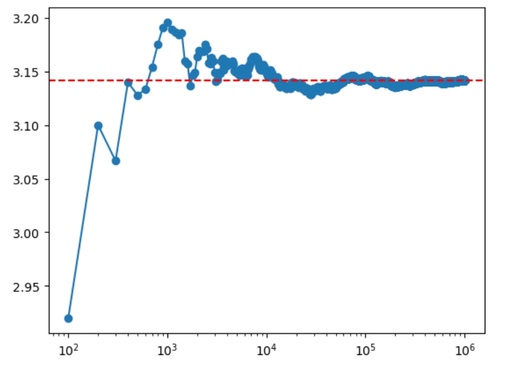
This will give you a very approximate volume of the 2D sphere, or an area of a circle. For more accurate results we need to use N=100_000.

Converging of the Monte-Carlo method for calculation of the surface area of the 2D circle. A circle surface can be considered as a volume of a 2D sphere.
Original image: 920 x 657
This image shows an approximate result of the program calculation. Because I do not fix the start value for a random generator, your picture will be different.
5-dimensional sphere
nothing will change if we will go to any other dimensions, so let's look at the 5-D sphere.
Really, the code will be almost the same, but I will show you some changes
square_size = 2
radius = 1
N = 1000000
dim = 5 # We will go for 5D case!!!!
The first change is to calculate the distance from the centre. It is a boring and not very scalable way to write squares for every dimension. We can use numpy features!
So, we generate a set of random dots, and then for every dot we calculate the distance from the centre. It can be possible to do with numpy by doing this along the axis.
points = np.random.uniform(-1, 1, size=(N, dim))
distances = (np.sum(points**2, axis=1))**0.5
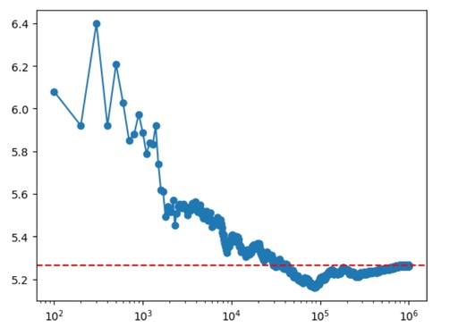
Also, I prefer to see, how results are approaching the ideal value and therefore I will recalculate the result every 100 trials
e_area = []
Nrange = np.arange(100, N+100, 100)
for n in Nrange:
    e_area.append(np.sum(inside[0:n])/n * square_size**dim)
The last step is to show the result. Also, I do prefer to use a logarithmic scale along the X-axis.
plt.plot(Nrange, e_area, marker='o')
plt.axhline(8/15*np.pi**2 * radius**dim, color='red', linestyle='--', label='Actual')
plt.xscale('log')
plt.show()
Converging of the Monte-Carlo method for calculation of the volume of the 5D-sphere. The result is in good agreement with the theory, where volume is equal 8*π2/15*R5
Original image: 920 x 657
N-dimensional ball
Now, because we are pretty confident in our Monte-Carlo technique, let's apply it to the calculation of the volumes of spheres of different dimensions.
The code will be the same with minor modifications. First of all, let's define parameters, with self-explanatory code.
square_size = 2
radius = 1
N = 1_000_000 # Max number of trials
Ndim = 20 # Max dimension for calculation
At this step, we will calculate the volume for each dimension from 2 towards Ndim (20 in our case). For each dimension, we will generate N dots in dim-dimensional space. It is easy to do with the Numpy random.uniform function.
Then we will check the location of every dot follow our algorithm as usual, and store the results.
e_area = []
d = []
for dim in range(2, Ndim+1):
    points = np.random.uniform(-1, 1, size=(N, dim))
    distances = (np.sum(points**2, axis=1))**0.5
    inside = distances <= radius
    e_area.append(np.sum(inside)/N * square_size**dim)
    d.append(dim)
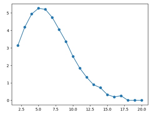
And now, let's plot the results.
plt.plot(d, e_area, marker='o')
plt.show()
Comparing of volumes of different dimension spheres with radius equal 1.
Original image: 920 x 657
In fact, it is not very correct to compare the volumes of spheres of a different dimension, because the units are different, and depends on the dimension of the system. But you can compare coefficients and also see, that the Monte-Carlo method can produce good results without knowing the exact equations. These are absolutely amazing results!
Published: 2023-11-28 00:55:01
Updated: 2023-11-28 22:34:08